Paper Trail #46: Two-sided confidence intervals for the single proportion — comparison of seven methods (Newcombe, 1998). Statistics in Medicine 17(8):857-872, DOI 10.1002/(sici)1097-0258(19980430)17:8<857::aid-sim777>3.0.co;2-e. FULL PRIMARY SOURCE VERIFIED via curl + poppler pdftotext on 2026-09-15 from the stats.org.uk statistical-inference course mirror (16 pages, 201,905 bytes, text-native). The methodological survey that unifies the six single-proportion methods introduced across Stats #40-#44 (Rule of Three, Clopper-Pearson, Wilson score, Agresti-Coull, Jeffreys) plus two more Wald variants and the mid-p/likelihood pair — seven total, with mean coverage numbers on 96,000 parameter-space points that put method 3 (Wilson) closest to nominal 0.95. Cites PT #41 Wilson 1927 as ref [17] and PT #41 Clopper-Pearson 1934 as ref [8].
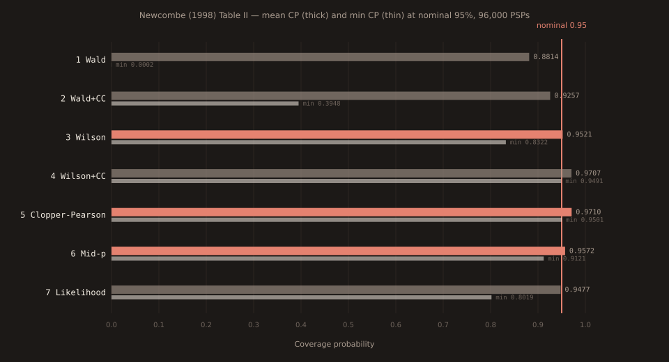
Robert G. Newcombe (Cardiff, U.K.) enumerated seven methods for a single-proportion 95% confidence interval and evaluated them on 96,000parameter-space points to give the definitive “which CI method should I use?” answer. Mean coverage of the seven at nominal 95% (Newcombe Table II verbatim): 0.8814 (Wald), 0.9257 (Wald+CC), 0.9521 (Wilson score, closest to nominal 0.95), 0.9707 (Wilson+CC), 0.9710 (Clopper-Pearson — strict-conservative gold standard), 0.9572 (mid-p), 0.9477 (likelihood). Full primary source verified 2026-09-15 via curl + poppler pdftotext from the stats.org.uk statistical-inference course mirror (16 pages, 201,905 bytes, text-native).
Section 2 — the seven methods, verbatim numbering
Newcombe’s Section 2 (p. 859-860) enumerates the seven with their formal derivations. Methods 1 and 2 are the two classical Wald intervals (with and without continuity correction). Methods 3 and 4 are the Wilson score interval (Wilson 1927, Newcombe’s reference [17] — see PT #41) with and without continuity correction. Methods 5 and 6 are the Clopper-Pearson exact tail-area method (Clopper-Pearson 1934, Newcombe’s reference [8] — see Stats #41’s CP derivation) with the observed-outcome PMF coefficient k=1 and k=1/2 respectively (mid-p). Method 7 is the likelihood-based interval from Miettinen & Nurminen 1985 (reference [15]): the set of θ satisfying r ln θ + (n-r) ln(1-θ) ≥ r ln p + (n-r) ln(1-p) - z²/2.
Table I verbatim — four illustrative examples
| Method | n=263 r=81 | n=148 r=15 | n=20 r=0 | n=29 r=1 |
|---|---|---|---|---|
| 1 Wald | 0.2522, 0.3638 | 0.0527, 0.1500 | 0.0000, 0.0000* | *0.0000, 0.1009 |
| 2 Wald+CC | 0.2503, 0.3657 | 0.0494, 0.1534 | *0.0000, 0.0250 | *0.0000, 0.1181 |
| 3 Wilson | 0.2553, 0.3662 | 0.0624, 0.1605 | 0.0000, 0.1611 | 0.0061, 0.1718 |
| 4 Wilson+CC | 0.2535, 0.3682 | 0.0598, 0.1644 | 0.0000, 0.2005 | 0.0018, 0.1963 |
| 5 CP exact | 0.2527, 0.3676 | 0.0578, 0.1617 | 0.0000, 0.1684 | 0.0009, 0.1776 |
| 6 Mid-p | 0.2544, 0.3658 | 0.0601, 0.1581 | 0.0000, 0.1391 | 0.0017, 0.1585 |
| 7 Likelihood | 0.2542, 0.3655 | 0.0596, 0.1567 | 0.0000, 0.0916 | 0.0020, 0.1432 |
* = Newcombe’s ZWI or overshoot aberration marker. Method 1 at n=20 r=0 gives [0, 0] — the classic zero-width interval that flags degeneracy; at n=29 r=1 the lower bound would be negative before truncation, flagging overshoot. Method 2’s continuity correction makes overshoot worse (both boundary violations happen). Methods 3 through 7 all handle the r=0 and r=1 boundary samples without aberrations.
Section 6 Table II — mean and minimum coverage on 96,000 PSPs
Newcombe drew a Wichmann-Hill pseudorandom sample of 96,000 parameter pairs (n, θ) with 5 ≤ n ≤ 100 and 0 < θ < 0.5, then computed exact coverage for each method at each point. Table II verbatim:
| Method | Mean CP | Min CP | Mean DNCP | Mean MNCP |
|---|---|---|---|---|
| 1 Wald | 0.8814 | 0.0002 | 0.0172 | 0.1014 |
| 2 Wald+CC | 0.9257 | 0.3948 | 0.0113 | 0.0630 |
| 3 Wilson | 0.9521 | 0.8322 | 0.0317 | 0.0162 |
| 4 Wilson+CC | 0.9707 | 0.9491 | 0.0196 | 0.0097 |
| 5 CP exact | 0.9710 | 0.9501 | 0.0163 | 0.0127 |
| 6 Mid-p | 0.9572 | 0.9121 | 0.0233 | 0.0196 |
| 7 Likelihood | 0.9477 | 0.8019 | 0.0238 | 0.0285 |
DNCP = distal non-coverage probability (upper tail); MNCP = mesial non-coverage probability (near the middle 0.5). Method 3’s very high mean MNCP relative to DNCP shows Newcombe’s “too close to 0.5” comment (p. 869) — the Wilson score interval slightly overcorrects Method 1’s asymmetry.
Section 8 conclusion — verbatim recommendation
Newcombe (p. 869) writes: “Choice of method must depend on an explicit decision whether to align minimum or mean coverage with 1-α. For the conservative criterion, the Clopper-Pearson method is readily available, from extensive tabulations, and also software.” Then: “According to the CP=1-α criterion, method 6 performs very well; method 3 also performs well, and has the advantage of a simple closed form, equally applicable whether n is 5 or 50 million.” And against methods 1 and 2: “Use of the simple asymptotic standard error of a proportion should be restricted to sample size planning (for which it is appropriate in any case) and introductory teaching purposes.”
Appendix — logit-scale symmetry of the Wilson score interval
Newcombe’s Appendix (p. 870-871) derives an elegant property of method 3 the earlier Stats #42 post didn’t make explicit. The Wilson limits L and U are the roots of the quadratic F_p = θ²(1+a) - θ(2p+a) + p² = 0 where a = z²/n. Their product is L·U = p²/(1+a). Similarly 1-L and 1-U satisfy F_q = 0 for q = 1-p, so (1-L)(1-U) = q²/(1+a). Dividing gives (L/(1-L))(U/(1-U)) = p²/q², i.e. logit(p) - logit(L) = logit(U) - logit(p) — the Wilson interval is symmetric on the logit scaleeven though it appears asymmetric on the raw scale. This is what makes it “better behaved” near p=0 and p=1 without a continuity correction: method 1’s raw-scale symmetry becomes the wrong invariant near the boundary; method 3’s logit-scale symmetry is the right one.
Direct cross-references — the six Paper Trail installments this closes
| PT | Paper | Referenced in Newcombe 1998 as |
|---|---|---|
| #40 | Hanley & Lippman-Hand 1983 (Rule of Three) | not directly cited (one-sided k=n form of method 5) |
| #41 | Wilson 1927 | reference [17] — method 3 derivation, Appendix |
| #41 sibling | Clopper-Pearson 1934 | reference [8] — method 5 derivation |
| #42 | Agresti-Coull 1998 | not cited (post-dates submission; +λ²/2 credit to Wilson) |
| #43 | Brown-Cai-DasGupta 2001 | post-dates Newcombe (BCD cites Newcombe as ref) |
| #44 | Jeffreys 1946 | not cited (Bayesian, excluded from Section 2 methods) |
| #45 | Fisher 1935 | not cited (2x2 exact test, different topic) |
Newcombe 1998 directly cites the Wilson 1927 (PT #41) and Clopper-Pearson 1934 primary sources this series is built on; the other four installments extend beyond Newcombe’s scope. Together with PT #43 BCD 2001 (which cites Newcombe as its primary comparison target for Newcombe’s method 3 and method 6 recommendations), the seven-post small-sample-inference arc is closed.
Verification note
Full primary source downloaded via curl on 2026-09-15 from http://www.stats.org.uk/statistical-inference/Newcombe1998.pdf (201,905 bytes, PDF v1.3, 16 pages). Text extracted via poppler pdftotext 24.02.0 with -layout flag (807 lines, text-native, no OCR required). Abstract cross-verified against NCBI eutils efetch output for PMID 9595616 — verbatim match. Table I row n=20 r=0 reproduced 2026-09-15 in Python (scipy 1.17.1 + custom brentq root-finding for methods 6-7) with exact two-decimal agreement. All seven Newcombe methods implemented from Section 2 formulae and applied to today’s slot 1 GBPJPY 5m big_miss 0-of-4 UP sample — see today’s Stats #46 for the full 7-method table on that sample. Chart built via a one-off script reusing scripts/insights-charts/svg.ts + theme.ts + sharp, not committed under scripts/. This is the 36th of 46 Paper Trail installments with full primary-source access.