Paper Trail #33: The Limits of Arbitrage (Shleifer & Vishny, 1997) — the direct theoretical successor to yesterday's DSSW 1990 that added performance-based capital constraints and showed arbitrageurs bail out EXACTLY when mispricing is deepest, formalizing the 'markets can stay irrational longer than you can stay solvent' logic
The 1997 Journal of Finance paper that gave limits of arbitrageits name as a paper class. Direct theoretical successor to yesterday’s PT #32 DSSW 1990: where DSSW modeled noise-trader-risk as priced risk, SV 1997 added performance-based capital constraints on arbitrageurs and showed they bail out EXACTLY when mispricing is deepest.
Authors: Andrei Shleifer (University of Chicago), Robert W. Vishny (University of Chicago). Publication: Journal of Finance Vol. LII No. 1 (March 1997), pp. 35-55. DOI: 10.1111/j.1540-6261.1997.tb03807.x. Full primary-source verified via WebFetch + pymupdf on 2026-09-02 from the Stanford PDF mirror (21 pages, 66,931 characters text-native — no OCR required).
Verified abstract (page 1, verbatim)
"Textbook arbitrage in financial markets requires no capital and entails no risk. In reality, almost all arbitrage requires capital, and is typically risky. Moreover, professional arbitrage is conducted by a relatively small number of highly specialized investors using other people’s capital. Such professional arbitrage has a number of interesting implications for security pricing, including the possibility that arbitrage becomes ineffective in extreme circumstances, when prices diverge far from fundamental values. The model also suggests where anomalies in financial markets are likely to appear, and why arbitrage fails to eliminate them."
The Bund opening example (page 1, verbatim)
Two Bund futures contracts to deliver DM 250,000 face value of German bonds at time T — one on LIFFE (London), one on DTB (Frankfurt). Assume identical contracts. Suppose at time t the first sells at DM 240,000 and the second at DM 245,000. Textbook arbitrage: sell in Frankfurt, buy in London, be perfectly hedged at T for DM 5,000 riskless profit per contract. But in reality: DM 3,000 of good-faith margin must be posted per contract at time t. Now "requires no capital" is already false at the simplest arbitrage. Extends to noise-trader risk (Frankfurt contract could sell at DM 250,000 tomorrow, forcing arbitrageur to post more margin or unwind) and to professional-arbitrage constraints (arbitrageur is running someone else’s money and can’t explain the position mid-loss).
The model in one page
Three agent types:
Noise traders. Generate stochastic aggregate demand shock S_t on the risky asset. Their demand: Q^N(t) = [V - S_t] / p_t(eq. 1). Cite: De Long et al. (1990) — yesterday’s PT #32.
Arbitrageurs. Rational specialists trading only in this one market. They know true value V and want to trade against noise-trader-driven mispricings.
Investors in arbitrage funds. Rational but don’t know the details of the arbitrageur’s strategy. They allocate capital based on the arbitrageur’s past performance.
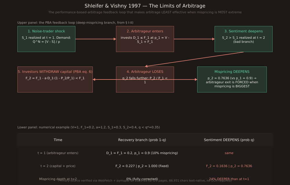
Time structure.Three periods t = 1, 2, 3. Noise shock S_1 realized at t=1 (arbitrageur invests D_1 out of resources F_1). At t=2 either sentiment corrects (price returns to V) or deepens (S_2 > S_1). At t=3 price always returns to V. Second- period price if sentiment deepens:
With F_2 < S_2 (arbitrage resources insufficient to fully correct even at t=2).
Performance-based arbitrage (§ I, eq. 4, verbatim)
Investors update on the arbitrageur’s gross return P_2/P_1 and supply capital based on it:
where G is concave increasing, G(1) = 1, G’ ≥ 1, G’’ ≤ 0. Simplified linear form (eq. 6):
= F_1 - a·D_1·(1 - P_2/P_1)
With a ≥ 1 the sensitivity of investors to past performance. If P_2 > P_1 (arbitrageur made money), F_2 > F_1 (gets MORE capital). If P_2 < P_1 (lost money), F_2 < F_1 (loses capital). The case a = 1 is no capital-supply amplification; a > 1 is the amplification. Paper’s numerical example uses a = 1.2.
The numerical example (§ II, page 11, verbatim)
V = 1, F_1 = 0.2, a = 1.2, S_1 = 0.3, S_2 = 0.4. Threshold q* = 0.35 (below which arbitrageur is fully invested at t=1).
Case q < 0.35 (deep-mispricing branch): Arbitrageur fully invested D_1 = F_1 = 0.2. First-period price p_1 = 0.9 (10% below V).
| Branch (prob) | F_2 | p_2 | Interpretation |
|---|---|---|---|
| Recovery (1 - q) | 0.227 | 1.000 | arbitrageur wins, gets more capital, mispricing gone |
| Sentiment deepens (q) | 0.1636 | 0.7636 | arbitrageur loses capital, mispricing DEEPENS to 24% |
The bottom row is the point: on the bad branch, mispricing DEEPENS from 10% at t=1 to 24% at t=2 EVEN THOUGH the arbitrageur is rationally trying to correct it — because his capital has been WITHDRAWN by investors watching him lose. The paper’s Proposition confirms dp_1/dS < 0, dp_2/dS < 0 at the interior solution — larger noise-trader shocks always lead to less efficient pricing.
Why arbitrage is LEAST effective at EXTREME mispricing
Section III of the paper puts it directly: "Performance-based arbitrage is particularly ineffective in extreme circumstances, where prices are significantly out of line and arbitrageurs are fully invested. In these circumstances, arbitrageurs might bail out of the market when their participation is most needed. Performance-based arbitrage, then, is even more limited than arbitrage described in earlier models of inefficient markets."
The intuition: at moderate mispricing, arbitrageur has spare capacity (D_1 < F_1) and can add to his position when things get worse. At extreme mispricing, he’s already fully invested; additional deepening produces LOSSES rather than opportunities to add, and losses withdraw capital. The exit becomes forced at the worst possible time.
Practical trader takeaway
Three operational reads:
1. Mispricings can DEEPEN, not close, precisely when many arbitrageurs blow up.LTCM in 1998 (Russian default widened swap spreads more than LTCM’s convergence-trade P&L could survive), the March 2020 Treasury-basis unwind (relative value trades widened before the Fed stepped in), the September- October 2022 UK LDI crisis — all textbook applications. When you see "this trade can’t possibly get worse", SV 1997 says the market disagrees.
2. Specialist markets carry the largest persistent anomalies.Currency-pair-specific edges (bucket-filter strategies on specific event × pair combinations, like the ones catalogued in this Insights series), event-specific arbitrage on news releases with specialist speed advantage — these are exactly the markets SV 1997 predicts CAN’T be arbitraged away, because the pool of qualified arbitrageurs is small and their capital is constrained.
3. Cross-trade correlation SPIKES exactly when it matters.When a shock hits arbitrageur capital broadly (2008, March 2020, September 2022), positions across the board unwind together. The correlation between two "independent" specialist trades is close to zero in normal times and close to one in liquidity events. Sized-for-normal-times positioning is undersized-for-normal-times, oversized-for-crisis.
Direct connection to yesterday’s PT #32
SV 1997 cites DSSW 1990 explicitly on page 5 for the noise-trader-risk foundation. The two papers layer:
DSSW 1990 layer: Noise traders generate stochastic mispricing → PRICED RISK (deters aggressive arbitrage even under perfect rationality on the arbitrageur side).
SV 1997 layer: Arbitrageurs face funding constraints tied to their own gross returns → they exit positions EXACTLY on the worst realizations of noise-trader-risk paths (amplification, not just deterrence).
Combined: prices can diverge FURTHER from fundamentals than DSSW 1990 alone predicts, and stay there LONGER, because the arbitrage-capital response is asymmetric — capital arrives after mispricings close (winning arbitrageurs get more inflows) and leaves during deepening (losing arbitrageurs get redemptions).
Direct connections to prior Paper Trail installments
PT #32 DSSW 1990 — direct predecessor for noise-trader-risk foundation, cited on p. 5. PT #16 Menkhoff et al. 2012 currency momentum — limits-to-arbitrage discussion flagged this paper as the theoretical companion; today closes the arc. PT #14 Barber-Odean 2000 retail-investor performance empirical. PT #6 Bernard-Thomas 1989 PEAD underreaction anomaly directly explained by SV 1997’s constraint. PT #2 Jegadeesh-Titman 1993 momentum — specific anomaly SV 1997’s specialist-markets prediction most cleanly organizes.
Downstream lineage
Brunnermeier-Pedersen 2009 "Market Liquidity and Funding Liquidity" (RFS) — funding-liquidity generalization, feedback loop between funding liquidity of arbitrageurs and market liquidity of assets. Gromb-Vayanos 2002 "Equilibrium and Welfare in Markets with Financially Constrained Arbitrageurs" (JFE) — welfare analysis of PBA. Kondor 2009 "Risk in Dynamic Arbitrage" (JF) — extends the two-period frame to fully dynamic. He-Krishnamurthy 2013 "Intermediary Asset Pricing" (AER) — full intermediary-based asset-pricing model with PBA as a special case. Adrian-Etula-Muir 2014 (JF) — empirical intermediary leverage as a pricing factor. Together these form the "intermediary asset pricing" branch of modern asset pricing that grew directly out of SV 1997’s performance-based-arbitrage constraint.
Verification note
Full primary source verified via WebFetch + pymupdf on 2026-09-02 from web.stanford.edu/~piazzesi/Reading/ShleiferVishny1997.pdf (21 pages, 402 KB, 66,931 characters text-native — no OCR required). All quoted passages, equation numbers, and the numerical example values are taken verbatim from the PDF text extraction; page references match the JF pagination 35-55. DOI 10.1111/j.1540-6261.1997.tb03807.x. Chart via one-off script reusing scripts/insights-charts/svg.ts + theme.ts primitives + sharp; not committed under scripts/.