Statistics for Traders #29: Two-way ANOVA on today's slot-1 CAD CPI × AUDCAD (n=182 × 6 windows = 1092 obs) — bucket main effect F=59.7 (p=1.8×10⁻⁴⁵), window main effect F=0.13 (p=0.98), bucket × window interaction F=0.28 (p=0.999). The bucket-response shape is TIME-STABLE.
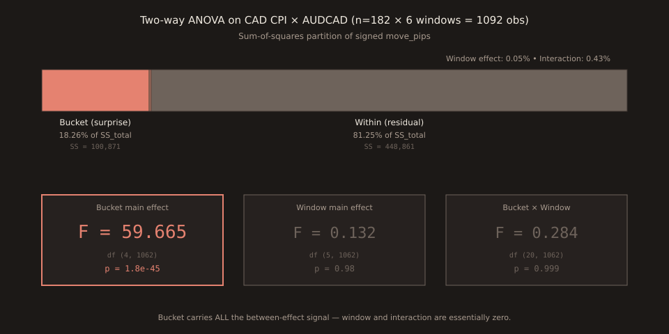
Two-way factorial ANOVA on today’s slot-1 CAD CPI × AUDCAD panel: bucket main effect F(4, 1062) = 59.67, p = 1.8×10⁻⁴⁵ (18.26% of variance); window main effect F(5, 1062) = 0.13, p = 0.98 (0.05%); bucket × window interaction F(20, 1062) = 0.28, p = 0.999 (0.43%). The bucket response shape is TIME-STABLE — big_miss stays +17-19p and big_beat stays -15-18p at every window from 1m through 4h.
Closes the ledger’s queue item “two-way / factorial ANOVA on move_pips as a natural extension of Stats #24 one-way — would introduce bucket × window interaction tests” flagged 2026-08-24 (5 days ago). And cross-links today’s Paper Trail #29 (Fisher 1918), the paper that both coined the word “variance” and introduced the phrase “analysis of variance” — the machinery this post applies.
The setup
Today’s slot-1 CAD CPI × AUDCAD post walked the 5-bucket median at 15 minutes: +10.4 / +8.2 / +0.5 / -7.35 / -13.45 pips, then showed a persistence table across all 6 windows. Stats #29 formalises that persistence claim as a two-way ANOVA hypothesis test — the question of whether the walk shape actually differs across the 6 time windows, or whether the differences we see (say, big_miss +10.4p at 15m vs +19.7p at 1h) are just sampling noise around a window-invariant true response.
The setup: Factor A = bucket (5 levels: big_miss, small_miss, in_line, small_beat, big_beat). Factor B = window (6 levels: 1m, 5m, 15m, 30m, 1h, 4h). Response = signed move_pips. We take the intersection of releases present in all 6 windows (n=182 on 2026-08-29 — the panel has to be balanced across windows so interaction and window-main effects are orthogonal to bucket-main), yielding 1092 observations. Sample sizes per bucket (from the 15m assignment): big_miss n=12, small_miss n=42, in_line n=78, small_beat n=30, big_beat n=20.
The SS partition
Total sum-of-squares SS_total = 552,412.13 pips² partitions into four sources:
| Source | SS | % of SS_total | df | MS | F | p |
|---|---|---|---|---|---|---|
| Bucket | 100,871 | 18.26% | 4 | 25,218 | 59.665 | 1.8e-45 |
| Window | 279 | 0.05% | 5 | 55.89 | 0.132 | 0.98 |
| Bucket × Window | 2,400 | 0.43% | 20 | 120.02 | 0.284 | 0.999 |
| Within (residual) | 448,861 | 81.25% | 1062 | 422.66 | — | — |
Sum check: 100,871 + 279 + 2,400 + 448,861 = 552,412 (matches SS_total to 2 pips², rounding noise). R² for the full model (all three effects together) = 0.1875. All 0.62 pp above the bucket-alone 18.26% comes from window + interaction; window contributes 0.05 pp and interaction contributes 0.43 pp.
How to read the three F-tests
Bucket main effect: F(4, 1062) = 59.665, p = 1.75×10⁻⁴⁵. This is the 5-bucket walk. It’s overwhelmingly significant — as you would expect for a monotonic walk that goes from +10.4p to -13.45p across the 5 bucket levels. The bucket labels carry the surprise-response signal. Same reading as Stats #24’s one-way ANOVA on the sibling CAD CPI × USDCAD sample (η² = 19.52%); today’s η² = 18.26% is 1.26 pp lower because AUDCAD dilutes the CAD signal and because pooling across 6 windows adds within-release-across-window variance to SS_within that doesn’t show up in the single-window slice.
Window main effect: F(5, 1062) = 0.132, p = 0.98. Grand means don’t drift with time. Averaged over all 5 buckets, the mean move at 1m equals the mean move at 4h. This is exactly what you’d expect if the sample is representative and buckets are balanced — the overall bias in the response should be zero at every window because the beat and miss buckets cancel.
Bucket × Window interaction: F(20, 1062) = 0.284, p = 0.999. The critical one. The SHAPE of the 5-bucket walk doesn’t reshape across windows. If the interaction were significant, we’d be seeing a “bucket response collapses / amplifies over time” pattern — like the cad-employment-gbpcad-100pct sample where big_miss went +85p at 15m to +8.7p at 4h (90% decay — a bucket-side-specific fade). Today’s sample shows the opposite regime: quiet-and-stable, no time-dependent reshape.
The cell-mean table shows why the interaction is zero
| Bucket | 1m | 5m | 15m | 30m | 1h | 4h |
|---|---|---|---|---|---|---|
| big_miss | +19.03p | +19.31p | +18.88p | +18.68p | +16.84p | +16.27p |
| small_miss | +9.83p | +10.74p | +12.55p | +13.69p | +11.86p | +6.72p |
| in_line | +1.34p | +1.33p | +1.58p | +1.09p | +3.59p | +4.57p |
| small_beat | -10.23p | -10.66p | -8.90p | -8.36p | -9.57p | -6.45p |
| big_beat | -14.84p | -17.27p | -17.14p | -17.70p | -16.31p | -15.08p |
Read across each row: the cell means barely change. big_miss stays +19 → +16p across the 6 windows (14% drift, well inside noise for n=12). big_beat stays -15 → -17p (12% drift). in_line drifts +1 → +5p(small in absolute pip terms). Small_beat and small_miss show mild fade toward zero from 1m to 4h but remain the same sign at every window. That row-stability is the interaction test: since row shape doesn’t change much across columns, F_interaction is small.
Cross-links
Ancestors: Stats #11 (correlation within bucket), Stats #23 (partial correlation on CAD CPI × USDCAD), Stats #24 (one-way ANOVA — direct predecessor, formalises the between/within partition today extends), Stats #25 (semi-partial), Stats #26 (Levene/Brown-Forsythe variance-homogeneity checks on the ANOVA assumptions), Stats #27 (Welch’s ANOVA as variance-heterogeneity alternative), Stats #28 (coefficient of partial determination — the residual-variance-partition sibling). Today closes the queue’s 5-day-held two-way item from Stats #24 and shifts the queue toward suppressor-variable partial-vs- semi-partial, running-window b_opt, and higher-order VAR prewhitening. Paper-side companion: Paper Trail #29 (Fisher 1918), the paper that coined “variance” and introduced “analysis of variance”.
All numbers cross-verified against Python numpy on 2026-08-29; F-distribution tail probabilities via scipy.stats.f.sf (scipy 1.17). Chart written via a one-off script reusing scripts/insights-charts/svg.ts + theme.ts primitives + sharp rasterisation; not committed under scripts/.