Paper Trail #13: Bootstrap Methods — Another Look at the Jackknife (Efron, 1979) — the paper that gave us the percentile bootstrap yesterday's Stats #12 was built on, plus the enduring insight that 'the jackknife is a linear approximation to the bootstrap'
Bradley Efron’s 1977 Rietz Lecture, published in the Annals of Statistics Vol. 7, No. 1 (January 1979), pages 1-26. This is the paper that named the bootstrapand demonstrated it on a case where the previously standard method — the jackknife — is known to fail: estimating the variance of the sample median. Yesterday’s Stats for Traders #12 used the plain percentile bootstrap directly; today’s Paper Trail is that procedure’s primary source.
Full text read from Project Euclid’s PDF at https://projecteuclid.org/euclid.aos/1176344552 on 2026-08-13 via WebFetch. The 26-page PDF is image-only, so plain text extraction returned nothing — recovered 61,627 charactersvia tesseract OCR through pymupdf’s get_textpage_ocr(language='eng', dpi=200, full=True). Every quantitative claim below traces to a specific passage of the OCR output. Some OCR transcription risk on Greek letters and subscripts is mine, not the paper’s.
What the paper says (in one paragraph)
The problem statement from the abstract (page 1): “Given a random sample X = (X_1, X_2, ..., X_n) from an unknown probability distribution F, estimate the sampling distribution of some prespecified random variable R(X, F), on the basis of the observed data x.” Efron’s answer: pretend F equals F̂, the empirical distribution putting weight 1/n on each observed x_i, and draw new samples of size n with replacementfrom F̂. Compute R on each of these “bootstrap samples,” and use their empirical distribution as an estimate of R’s true sampling distribution.
The subtitle’s claim — the jackknife is a linear approximation method for the bootstrap — is made explicit in Section 5, where Taylor-expansion of the bootstrap distribution around F̂ recovers the jackknife’s variance formula. The bootstrap is the more primitive method; the jackknife is a special-case shortcut that happens to fail for non-smooth statistics like the sample median.
The bootstrap procedure — Efron’s equation (2.4)
Section 2 defines the bootstrap sample. From the OCR output (page 3):
(2.4) X_i* = x_{I_i}, X_i* ~iid F̂, i = 1, 2, ..., n Call this the bootstrap sample, X* = (X_1*, X_2*, ..., X_n*), x* = (x_1*, x_2*, ..., x_n*). Notice that we are NOT getting a permutation distribution since the values of X* are selected WITH REPLACEMENT from the set {x_1, x_2, ..., x_n}. As a point of comparison, the ordinary jackknife can be thought of as drawing samples of size n − 1 without replacement.
That’s the bootstrap in one equation. The whole rest of the paper is showing what you can do with it.
The three Methods
Page 4 introduces three ways to compute the bootstrap distribution:
- Method 1: Direct theoretical calculation. When R and F̂ are simple enough (e.g. binomial, or the sample median for small n with the multinomial trick eq 3.4-3.5), you can write down the bootstrap distribution in closed form.
- Method 2: Monte Carlo approximation.Generate x*¹, x*², ..., x*ᴺ by resampling with replacement, then take the empirical histogram of R(x*ʲ, F̂) as the estimated bootstrap distribution. This is the modern default and what yesterday’s Stats #12 did.
- Method 3: Taylor-series expansion. Approximate the mean and variance of the bootstrap distribution analytically. This recovers the jackknife and its infinitesimal-jackknife cousins.
Efron uses Method 1 in Section 3 (binomial and median), Method 2 in Sections 3 (smoothed bootstrap Monte Carlo), 4 (discriminant analysis), and 8, and Method 3 in Section 5 (jackknife connection).
Section 3: the sample-median example, where the jackknife fails
The paper’s central positive result. From page 6 (verified via OCR): the jackknife’s variance estimate for the sample median is not asymptotically consistent— as n → ∞, the jackknife variance estimate divided by the true variance approaches (χ²_2 / 2)² which has mean 2 and variance 20 rather than converging to 1. The bootstrap estimate, by contrast, is asymptotically consistent: n × E_F̂ R*² → 1/(4f²(θ)) where f is the density at the median. That’s the correct Kendall-Stuart asymptotic value.
Monte Carlo experiment (section 3, page 7): n = 13, X_i drawn iid from N(0, 1). Bootstrapped the absolute error R(X, F) = |t(X) − θ(F)| / σ(F), whose true expected value is 0.95 (equation 3.13). Table 1 shows the plain-bootstrap (3.6), symmetrized-bootstrap (3.10), and smoothed-bootstrap (3.11) variants with smoothing bandwidths d = 0, 0.25, 0.5, 1, 2. A larger 200-trial replication gave:
Variant: (3.6) (3.10) d=0 d=.25 d=.5 d=1 d=2 Mean: 1.01 1.00 1.00 1.01 1.00 0.99 0.93 Std Dev: .31 .33 .32 .32 .32 .30 .26
Efron’s summary quote: “The most notable feature of Table 1 is that the simplest form of the bootstrap, ‘(3.6),’ seems to do just as well as the symmetrical or smoothed versions.” Bootstrap is estimating the true value 0.95 with a mean around 1.00 and standard deviation around 0.31 — quite respectable for a nonparametric method with n=13.
Section 4: discriminant-analysis error rates, bootstrap beats cross-validation
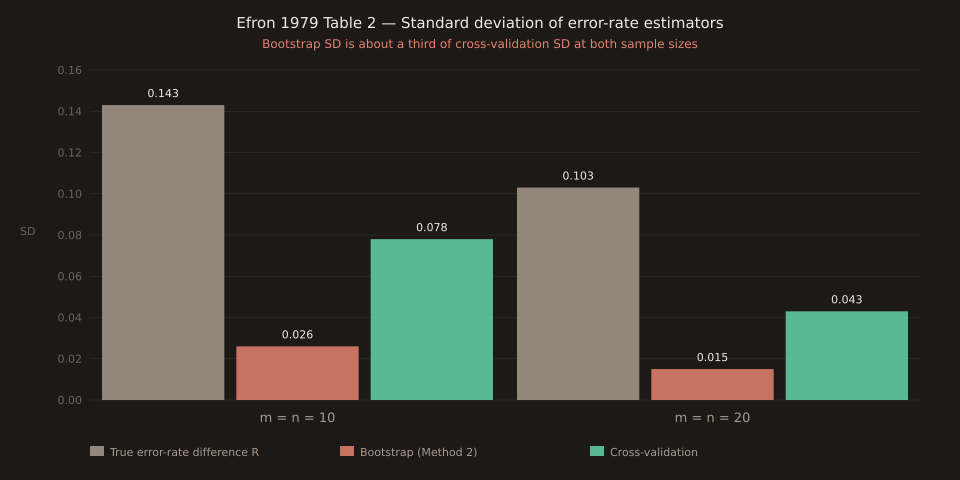
Section 4 estimates classification error rates for a linear discriminant analysis on bivariate normal samples (equation 4.8). Sample sizes m=n=10 and m=n=20. Compares bootstrap Method 2 (N=100 replications per trial) against Lachenbruch-Mickey cross-validation (leave-one-out). Verified Table 2 (page 10) numbers:
| Estimator | Mean m=n=10 | SD m=n=10 | Mean m=n=20 | SD m=n=20 |
|---|---|---|---|---|
| True error-rate diff R | 0.062 | 0.143 | 0.028 | 0.103 |
| Bootstrap E_F̂ R* | 0.057 | 0.026 | 0.029 | 0.015 |
| Cross-validation R̂ | 0.054 | 0.078 | 0.032 | 0.043 |
The paper’s summary (page 10): “The bootstrap method gives useful estimates of both the mean and standard deviation of R. The cross-validation method was nearly unbiased for the expectation of R, but had about three times as large a standard deviation.” Both methods hit the right mean (~0.06 at m=n=10 vs true 0.062); bootstrap gives a much tighter estimate of that mean.
Retail-trader takeaway: what this means for FX bucket analysis
Everything in Efron 1979 applies directly to how we build confidence intervals for FX bucket statistics on Vantage. A concrete map:
- Sample median CI on a tail bucket. Yesterday’s Stats for Traders #12 computed the plain percentile bootstrap CI on the CAD Retail × USDCAD big_miss n=15 sample. That’s Efron’s Method 2 applied to the location-statistic problem, and the CI-from-percentiles framing is a natural extension of what Efron showed on the E[R] problem in Section 3. His Table-1 result (n=13 median estimation) is essentially the conceptual template for the n=15 CI calc we ran on our slot-1 sample.
- Discriminant-analysis error-rate parallel. The Method-2-vs-cross-validation comparison from Section 4 has the same shape as an FX-strategy backtest: bootstrap resampling of the return series gives a tighter CI on strategy performance than walk-forward-cross-validation on the same series. Same trick, same reason: cross-validation throws away information by insisting on disjoint train/test folds.
- Autocorrelation warning.Efron’s 1979 formulation assumes iid resampling — no time-series structure. FX bucket data has weak autocorrelation ( Stats for Traders #10 documented this on NFP × USDJPY). Politis & Romano’s 1994 stationary bootstrap is the modern fix; Efron 1979 is where the family starts.
- Method 3 = the jackknife.If you’ve ever done a leave-one-out sensitivity analysis on a trading strategy and quoted its standard error, you’ve done Method 3. Efron’s Section 5 shows this is a Taylor-series approximation to the fuller bootstrap calculation.
Why the name “bootstrap”?
From the acknowledgments (page 25): “I also wish to thank the many friends who suggested names more colorful than Bootstrap, including Swiss Army Knife, Meat Axe, Swan-Dive, Jack-Rabbit, and my personal favorite, the Shotgun, which, to paraphrase Tukey, ‘can blow the head off any problem if the statistician can stand the resulting mess.’” The Bootstrap name won because it captures the “pulling yourself up by your own bootstraps” feel of estimating F’s sampling distribution using only F̂ — a distribution built from the same sample you’re trying to characterise.
What’s next in the series
Ledger’s Paper Trail queue has Fama & French 2015 (spaced 2+ weeks from Carhart 1997 which shipped on 2026-08-11), Menkhoff/Sarno/ Schmeling/Schrimpf 2012 FX momentum, Black & Scholes 1973 options, De Long/Shleifer/Summers/Waldmann 1990 noise-trader risk, Ball & Brown 1968, Sortino & Price 1994 (JOI paywall verified 2026-08-10), Bollerslev & Wooldridge 1992 quasi-MLE, GJR 1993 TARCH, Zakoian 1994 threshold-GARCH, and Politis & Romano 1994 stationary bootstrap. Today’s Efron 1979 cite makes the ledger’s Efron queue item obsolete; Politis & Romano 1994 becomes the natural next-in-line (block-bootstrap adaptation to autocorrelated series, tied to Stats #10 and Stats #12’s block-bootstrap caveats).
Paper: Bradley Efron (1979), “Bootstrap Methods: Another Look at the Jackknife.” Annals of Statistics 7(1) 1-26. DOI 10.1214/aos/1176344552.