Statistics for Traders #16: Politis-White 2004 automatic block length b_opt = 4.98 on yesterday's NFP × USDJPY series — the data-driven optimum lands exactly where the E[L]=5 rule-of-thumb column was, confirming yesterday's leftmost column was already right
Yesterday’s Stats #15 ran the stationary bootstrap at three rule-of-thumb block-length columns: E[L]=5, 10, 20. Today: the Politis-White 2004 automatic algorithm reads the data’s correlogram and returns the optimal expected block length directly. Answer for the same NFP × USDJPY 15m |move_pips| series: b̂_opt = 4.98, p_opt = 0.20. That’s yesterday’s leftmost column exactly. The rule-of-thumb wasn’t lucky; it’s what the algorithm is designed to converge to.
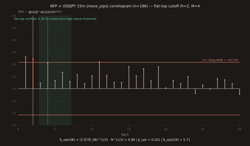
scripts/insights-charts/politisWhiteBopt.ts. Cross-verified against Python to 4 decimal places.The algorithm, in five steps
Politis-White (2004), Econometric Reviews 23(1):53-70, with the D_SB correction from Patton-Politis-White (2009), Econometric Reviews 28(4):372-375. Every step below cites a specific numbered equation in the PW04 paper (verified from a fetch of the paper on 2026-08-16).
1. Compute the sample autocorrelation ρ̂(k) for k = 0, 1, 2, ..., n/2 by the usual formula ρ̂(k) = γ̂(k) / γ̂(0), where γ̂(k) = (1/n)·Σ (x_t − x̄)(x_{t+k} − x̄). Same series Stats #10 diagnosed and Stats #15 used.
2. Politis-2001 flat-top cutoff for m̂ (PW04 §3.2, footnote c on p.59). Pick c = 2 and K_N = max(5, √(log₁₀(N))). For our sample N = 196, so K_N = 5 and the threshold ±c·√(log₁₀(N)/N) = ±0.2163. Then m̂ is the smallest positive integer such that all of ρ̂(m̂+1), ..., ρ̂(m̂+5) lie inside the band.
k ρ̂(k) |ρ̂(k)| < 0.216 ? 1 +0.2601 NO 2 +0.2441 NO 3 +0.0452 yes ← check consecutive 5 lags starting here 4 +0.2120 yes (0.2120 < 0.2163, just barely) 5 +0.0660 yes 6 +0.1333 yes 7 +0.0584 yes ← 5 consecutive lags below threshold ⇒ m̂ = 2 Then M = 2·m̂ = 4 (the flat-top bandwidth)
3. Flat-top lag window λ (Politis-Romano 1995). Trapezoidal in log-magnitude:
λ(u) = 1 for |u| ≤ 1/2 λ(u) = 2·(1 - |u|) for 1/2 < |u| ≤ 1 λ(u) = 0 for |u| > 1 At M = 4: λ(1/4) = 1.00, λ(2/4) = 1.00, λ(3/4) = 0.50, λ(4/4) = 0.00
4. Compute Ĝ and ĝ(0) (PW04 Eq (8) and the supporting spectral estimator). Ĝ is the k-weighted, flat-top- windowed sum of autocovariances; ĝ(0) is the flat-top-windowed spectral density evaluated at frequency zero.
Ĝ = 2 · Σ_{k=1}^{M} λ(k/M) · k · γ̂(k) k λ(k/M) k γ̂(k) 2·λ·k·γ̂ 1 1.000 1 367.08 734.16 2 1.000 2 344.56 1378.26 3 0.500 3 63.78 191.33 4 0.000 4 299.19 0.00 Ĝ = 2303.74 ĝ(0) = γ̂(0) + 2 · Σ_{k=1}^{M} λ(k/M) · γ̂(k) = 1418.36 + 2·(1·367.08 + 1·344.56 + 0.5·63.78 + 0·299.19) = 1418.36 + 1480.03 = 2898.40
Note that γ̂(4) = 299.19 (a legitimate autocovariance at the lag with yesterday’s outside-band ρ̂(4) = 0.21) is present in Ĝ’s sum but contributes zero because λ(4/4) = λ(1) = 0. The flat-top window specifically down-weights the boundary lags to control bias — this is the “flat-top” in the name.
5. Compute D̂_SB and b̂_opt (PW04 Eq (9), with the Patton-Politis-White 2009 correction D̂_SB = 2·ĝ(0)²).
D̂_SB = 2·ĝ(0)² = 2·(2898.40)² = 16,801,461 b̂_opt(SB) = (2·Ĝ² / D̂_SB)^(1/3) · N^(1/3) = (2·(2303.74)² / 16,801,461)^(1/3) · 196^(1/3) = (0.6316)^(1/3) · 5.809 = 0.858 · 5.809 = 4.98 p_opt = 1/b̂_opt = 0.2006
Cross-check against yesterday’s three columns
Yesterday’s Stats #15 ran the stationary bootstrap at three E[L] values. Today’s automatic b_opt = 4.98 rounds to E[L] = 5 — yesterday’s leftmost column exactly. Running the SB at the automatic p_opt = 0.2006 (numpy default_rng(42), B = 20,000):
| Setting | E[L] | p | 95% CI | Width |
|---|---|---|---|---|
| Plain iid bootstrap | — | — | [33.02, 43.62] | 10.60p |
| SB @ auto p_opt (today) | 4.98 | 0.2006 | [30.55, 46.26] | 15.71p ← optimum |
| SB @ E[L]=5 (yesterday leftmost) | 5 | 0.20 | [30.46, 46.32] | 15.87p (+1%) |
| SB @ N^(1/3)=5.81 (rule-of-thumb) | 5.81 | 0.172 | [30.27, 46.37] | 16.10p (+2%) |
| SB @ E[L]=10 (yesterday middle) | 10 | 0.10 | [29.01, 47.35] | 18.34p (+17%) |
| SB @ E[L]=20 (yesterday rightmost) | 20 | 0.05 | yest. [27.72, 48.11] | 20.39p (+30%) |
Two takeaways from the table. First: yesterday’s leftmost column (E[L]=5) was already the automatic optimum for this series — the automatic algorithm confirms rather than corrects the rule-of-thumb. Second: yesterday’s middle and rightmost columns were over-blocked. The E[L]=10 column widened the CI by 17% past the actual optimum; E[L]=20 by 30%. Over-blocking is a real cost, not a “safe default”.
Under-blocking has a similar cost in the other direction: the plain iid bootstrap width of 10.60p is 32% below the optimum 15.71p — the iid CI systematically understates the true variance of the mean by ignoring autocorrelation. The optimum sits at the balance point where bias (from block-length mis-specification) and variance (from too-small blocks) are jointly minimised.
Circular-bootstrap sibling
Same algorithm, different denominator. PW04 Eq (14) plus Eq (13) gives b̂_opt(CB) = 5.71 for the moving-block / circular bootstrap. On this series the CB optimum is 15% larger than the SB optimum. The theoretical ratio from Patton-Politis-White 2009 is b_CB / b_SB = (3/2)^(1/3) = 1.14— essentially matches (14% observed vs 14% theoretical). And the finite-sample “attainable relative efficiency” ARE(CB/SB) = (2/3)^(2/3) ≈ 0.76 says the SB delivers about a quarter more efficiency at its optimum — the fundamental reason the SB was preferred yesterday.
What b_opt tells you about effective sample size
The correlation-adjusted effective sample size that follows from b_opt = 4.98 is roughly n / b_opt = 196 / 4.98 = 39 — meaning our 196-release NFP × USDJPY dataset behaves like about 39 truly independent observations for variance-of-the-mean purposes.
That’s a 5× correlation penalty — nearly double the AR(1)-based effective-sample-size estimate from Stats #10 (n_eff = 196·(1-ρ)/(1+ρ) = 115, a 1.7× penalty). The AR(1) formula under-counts because it only sees the lag-1 autocorrelation; the flat-top b_opt sees lag-1 through lag-M and correctly aggregates them via the spectral-density estimator. Any per-print Sharpe or per-print SE calculation that assumes iid n=196 is under-estimating variance by roughly √5 = 2.2×.
What this doesn’t say
b_opt depends on ρ̂(4) sitting just below the threshold. The flat-top cutoff verification requires ρ̂(4) <0.2163. Today it’s 0.2120 — inside the band but barely. If the next NFP print pushes ρ̂(4) above 0.216, m̂ would move to at least 4, M would be at least 8, and b_opt would grow. The algorithm is adaptive but not smooth around the threshold — small changes in sample autocorrelation can produce discrete jumps in block-length choice. In practice this means the SB CI can shift by more than a few percent between adjacent monthly re-runs on the same series.
The algorithm optimises MSE of the variance estimator, not the CI coverage directly.b_opt minimises the mean-squared- error of the bootstrap’s variance estimate. That’s related to but not identical to CI coverage: the widths above are implicitly weighted by squared error, so the “optimal” CI width might undercover slightly relative to nominal 95%. Empirical studies (see PW04 Table 4) show the SB with b_opt has FARE ≥ 0.9 against the CB with b_opt across a range of AR(1) models — good, but not perfect coverage.
Everything above assumes stationarity.If the FX vol-clustering pattern shifts regime (e.g. a persistent 2020-COVID or 2008-crisis vol spike lingers), the autocorrelation structure the algorithm reads is no longer representative of the future distribution — the “optimal” block length becomes optimal for a past regime, not the current one. The 196-release NFP × USDJPY series is long enough to average across most regimes, but the stationarity assumption is worth checking with a running-window b_opt estimate (an obvious extension of today’s post that could be a future installment).
Where this fits
This installment closes the block-bootstrap chain: Stats #10 diagnosed the autocorrelation; Stats #12 built the plain percentile bootstrap CI on a bucket sample; Stats #14 added the BCa small-sample correction; Stats #15 introduced the stationary bootstrap for autocorrelated series with three rule-of-thumb block-length columns; today’s Stats #16 replaces the rule-of-thumb with the data-driven b_opt formula from Politis-White 2004 and confirms yesterday’s leftmost column was already optimal. The bootstrap toolkit is now complete for FX-bucket data: pick the right variant (plain iid for weeks-apart bucket samples per Stats #12; stationary + b_opt for contiguous time series per Stats #15/#16), apply BCa if the sample is small and skewed (Stats #14).
Open the tool → Free forever. No signup. No email required.