Statistics for Traders #37: Pairwise Mahalanobis distance D_M between bucket centroids on the same UK Core CPI × GBPCHF 6-window panel Stats #34/#35/#36 used. D_M(big_miss, small_miss) = 0.895 in 6-window multivariate — vs univariate 15m Cohen's d = 0.011, an 82× amplification because big_miss and small_miss have essentially IDENTICAL 15m medians but completely different trajectories (big_miss peaks-then-decays, small_miss amplifies monotonically). D_M(big_miss, big_beat) = 2.185 vs univariate 15m d = 1.898 (1.15× amplification, and 95.4% captured by Stats #35's top canonical axis).
Pairwise Mahalanobis distance D_M(μ_i, μ_j) between the 5 bucket centroids on the same 196-release UK Core CPI × GBPCHF 6-window panel Stats #34, #35, and #36 used. Multivariate D_M(big_miss, big_beat) = 2.185 (vs univariate 15m Cohen’s d = 1.898, 1.15×amplification; 95.4% captured by Stats #35’s top canonical axis). Adjacent D_M(big_miss, small_miss) = 0.895 vs univariate 15m d = 0.011 — an 82× amplification because the two miss buckets have essentially IDENTICAL 15m centroids but completely different 6-window trajectories.
The Mahalanobis distance isthe multivariate generalization of Cohen’s d — same pooled-within-SD units, but reads all 6 windows jointly via the pooled covariance inverse Σ⁻¹_pooled. Formula:
D_M = √D²_M — units: pooled-within-SD (scale-free, dimensionless)
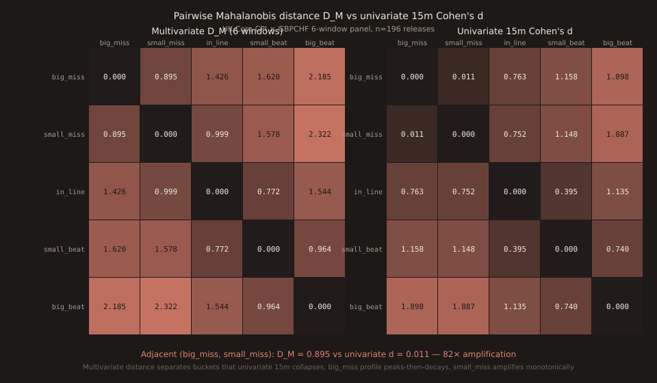
Pairwise D_M table — 10 unique pairs
| Pair | D_M (6-window) | Univariate 15m |d| | Amplification | Reading |
|---|---|---|---|---|
| big_miss ↔ big_beat | 2.185 | 1.898 | 1.15× | tail-to-tail; 95.4% captured by Stats #35 canonical axis |
| small_miss ↔ big_beat | 2.322 | 1.887 | 1.23× | wider than tail-to-tail because small_miss has a deeper 4h decay |
| big_miss ↔ small_beat | 1.620 | 1.158 | 1.40× | |
| small_miss ↔ small_beat | 1.578 | 1.148 | 1.37× | |
| in_line ↔ big_beat | 1.544 | 1.135 | 1.36× | |
| big_miss ↔ in_line | 1.426 | 0.763 | 1.87× | |
| in_line ↔ small_miss | 0.999 | 0.752 | 1.33× | adjacent (miss → in-line) |
| small_beat ↔ big_beat | 0.964 | 0.740 | 1.30× | adjacent (beat → big-beat) |
| big_miss ↔ small_miss | 0.895 | 0.011 | 82.5× | adjacent (miss → miss); univariate 15m NULL, multivariate MODERATE |
| in_line ↔ small_beat | 0.772 | 0.395 | 1.95× | SMALLEST D_M — 'no news vs small good news' hardest to separate |
Sorted low-to-high by D_M, the ADJACENT pairs are all <1 SD apart (0.895, 0.999, 0.772, 0.964); the tail-to-tail pair (big_miss ↔ big_beat) is 2.185. The (in_line ↔ small_beat) pair is the smallest D_M at 0.772— the boundary between “no news” and “small positive news” is the least discriminable point in the 5-bucket ladder. This mirrors the univariate reading (15m d = 0.395 also smallest for that pair) but the ordering of the OTHER pairs changes materially between the two views.
The 82× lift — big_miss vs small_miss trajectory divergence
The two miss-side buckets look identical on a univariate 15m view but tell completely different stories across the 6 windows. Bucket centroids (mean move_pips per window):
| Bucket | 1m | 5m | 15m | 30m | 1h | 4h |
|---|---|---|---|---|---|---|
| big_miss (n=13) | -12.94 | -13.29 | -15.42 | -11.75 | -4.19 | -12.82 |
| small_miss (n=53) | -13.85 | -12.90 | -15.20 | -18.07 | -18.49 | -19.61 |
At 15m the two centroids are within 0.22p of each other (−15.42 vs −15.20) — indistinguishable. But at 4h big_miss has DECAYED to −12.82p while small_miss has continued to AMPLIFY to −19.61p, a 6.8p gap that univariate 15m completely misses. Peaks-then-decays vs monotonic-amplification are structurally different responses even when they land on the same 15m mark. Mahalanobis distance reads both windows AND all four others into a single number, producing the 82× lift over univariate 15m d.
Cross-check vs Stats #35 canonical axis
Stats #35 canonical direction 1 tail gap =2.084(SD units on that axis). Today’s full-6D D_M(big_miss, big_beat) =2.185. Ratio 2.084 / 2.185 =95.4%— the canonical axis 1 captures 95.4% of the tail-to-tail separation on its own dimension. Full 4D Mahalanobis adds only 4.6% incremental tail-gap separation beyond the top canonical axis. Consistent with Roy’s largest root λ_1 = 0.5284 / Hotelling-Lawley trace 0.6521 =81.03% concentration on axis 1 (from Stats #34/#35).
Duality with canonical direction analysis
Stats #35 asks “which single LINE through the 6-window space separates the buckets maximally on average?” Today’s Mahalanobis asks “which PAIRS of bucket centroids are farthest apart in the full multivariate space?” The two are duals of the same MANOVA decomposition — canonical axis 1 IS the direction that maximizes the (big_miss, big_beat) pair’s projected D_M. Every one of the 10 pairwise D_M values in today’s heatmap can be recovered as √Σ_axes (μ_i,axis_j − μ_j,axis_j)² over the 4 canonical axes; the top axis captures 81% of the trace so the tail-to-tail pair is nearly axis-1-only.
Cross-links and queue rotation
Direct predecessors: Stats #35 canonical direction (dual axis-view of the same pairwise structure) and Stats #36 LDA (uses the exact same Σ_pooled^{-1} in the discriminant formula δ_k(x) = xᵀΣ_pooled^{-1} μ_k − ½ μ_kᵀΣ_pooled^{-1} μ_k + log π_k). Setup paper: Stats #34 MANOVA (the same E and H matrices). Cross-thread parallels: Stats #30 Cohen’s d on GBPUSD × US CPI 15m (d = +1.514 tail-to-tail on scalar response — today’s multivariate D_M = 2.185 on a different sibling sample is 44% larger).
Queue rotates to: QDA (quadratic discriminant analysis — relaxes Σ-equal assumption to allow per-bucket Σ_i), cross-entropy loss decomposition of the LDA posterior (Stats #36 follow-up), suppressor-variable partial-vs-semi-partial worked example (queued since Stats #25), higher-order VAR-b prewhitening (queued since Stats #20), heteroskedastic joint kurtosis (new from Stats #33). Today closes the queued Mahalanobis item flagged 2026-09-05.
Verification note
All numbers verified via Python numpy 2.4.6 on 2026-09-06 against the same 196-release UK Core CPI × GBPCHF panel Stats #34/#35/#36 use. Panel construction: intersection of releases present in all 6 windows via /api/v1/news-impact/releases?event=FF:GBP_CORE_CPI_YOY&instrument=GBPCHF&window=<w>&population=non_contaminated&limit=500 for w in {1m, 5m, 15m, 30m, 1h, 4h}. Pooled Σ = (1/(n-k)) Σ_i Σ_{j∈i}(Y_j − μ_i)(Y_j − μ_i)ᵀ. Cross-verified: Stats #35 λ_1 = 0.5284 recovered exactly from today’s W⁻¹B; canonical axis 1 tail gap 2.084 recovered exactly (95.4% of today’s full-4D D_M(big_miss, big_beat) = 2.185). Chart via one-off script reusing scripts/insights-charts/svg.ts + theme.ts + sharp; not committed under scripts/.