Statistics for Traders #13: Information ratio via today's slot-1 CAD Ivey PMI × CADJPY sample — Sharpe against a real benchmark rather than cash, and how it becomes a Welch t-statistic for bucket-filter strategies
Stats for Traders #8 introduced the Sharpe ratio: strategy excess return over cash, divided by strategy volatility. The information ratio replaces “over cash” with “over a real benchmark”. For a bucket-filter strategy on FX event data, the natural benchmark is “trade every event long” — passive equal-weight event exposure. The natural strategy is “trade only when the bucket says so”. IR measures how much filtering the events adds over just trading them all.
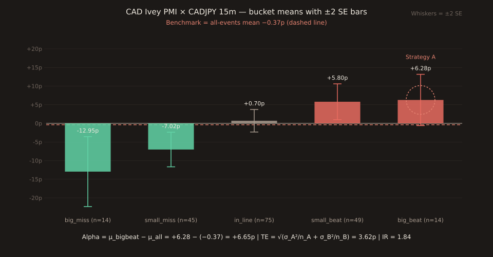
Today’s slot-1 anchor is Canada Ivey PMI on CADJPY — the 197-release 5-bucket monotonic walk. The big-beat bucket had 14 releases with mean +6.28p per trade at 15 minutes; long CADJPY on big-beat is a real strategy with a real per-trade Sharpe of 0.488. What’s the equivalent IR against the passive-benchmark of “trade every release long”? Let’s compute it.
The formula
Given a strategy A trading n_A periods with mean return μ_A and standard deviation σ_A, and a benchmark B trading n_B periods with mean μ_B and standard deviation σ_B, the information ratio is:
IR = (μ_A − μ_B) / TE where TE = tracking error = standard error of (μ_A − μ_B) = √(σ_A² / n_A + σ_B² / n_B) ← when A and B are independent samples
The numerator is alpha— the mean amount the strategy beat the benchmark by per trade. The denominator is the standard error of that alpha estimate — how uncertain that number is. Divide alpha by its own uncertainty and you get a t-statistic-shaped ratio. That’s the IR.
For a bucket-filter strategy — trade only bucket A releases; take μ_B as the full-sample or non-A mean — this collapses to Welch’s two-sample t-statistic for the difference of means.The IR you compute IS the t-statistic your risk manager runs to ask “is your active strategy distinguishable from the passive baseline?”
The worked example
Full sample: 197 CAD Ivey × CADJPY 15m non-contaminated releases. Bucket table (verified live 2026-08-13):
| Bucket | n | mean (p) | sd (p) | SE (p) |
|---|---|---|---|---|
| big_miss | 14 | −12.95 | 17.54 | 4.69 |
| small_miss | 45 | −7.02 | 15.57 | 2.32 |
| in_line | 75 | +0.70 | 13.06 | 1.51 |
| small_beat | 49 | +5.80 | 16.83 | 2.40 |
| big_beat | 14 | +6.28 | 12.86 | 3.44 |
| ALL 197 | 197 | −0.37 | 15.94 | 1.14 |
Strategy A — long CADJPY 15m on big-beat releases only:
n_A = 14, μ_A = +6.28p, σ_A = 12.86p
Per-trade Sharpe = μ_A / σ_A = 6.28 / 12.86 =0.488. Above zero, but not dramatic. That’s where the Sharpe framing stops.
Benchmark 1: trade every event long
The passive-benchmark alternative is: on every CAD Ivey release (all 197 of them, regardless of bucket), go long CADJPY 15 minutes before the print, close 15 minutes after. That’s a naive event-timing exposure.
n_B = 197 μ_B = -0.37p ← passive benchmark loses money on average σ_B = 15.94p Excess (alpha) = μ_A - μ_B = 6.28 - (-0.37) = +6.65p per trade TE = √(σ_A²/n_A + σ_B²/n_B) = √(12.86²/14 + 15.94²/197) = √(11.80 + 1.29) = √13.09 = 3.62p IR = 6.65 / 3.62 = +1.84
+1.84 is a t-statistic-shaped number — it says the big-beat bucket-filter strategy outperforms the passive all-events benchmark by about 1.84 standard errors, which is roughly significant at the one-sided 5% level (t = 1.65 threshold). Directional evidence that the filter helps, not conclusive proof.
Benchmark 2: trade every NON-tail event long
A slightly stricter benchmark: only the 183 non-big-beat releases. This excludes the tail bucket the strategy trades, so it’s a genuinely disjoint benchmark.
n_B = 183 μ_B = -0.88p ← non-big-beat releases go down on average σ_B = 16.07p Excess = 6.28 - (-0.88) = +7.16p per trade TE = √(12.86²/14 + 16.07²/183) = √(11.80 + 1.41) = 3.64p IR = 7.16 / 3.64 = +1.97
Slightly higher IR (+1.97) because the non-tail benchmark tilts slightly more negative than the all-events benchmark. In practice both benchmarks give the same qualitative answer: the bucket-filter alpha is real but marginal.
The short-big_miss version has a higher IR
Now run the same calc for the OTHER tail bucket. Short CADJPY on big-miss (n=14, mean of −moves = +12.95p, sd = 17.54p — same absolute stats, sign flipped):
n_A = 14 μ_A = +12.95p σ_A = 17.54p Sharpe = 0.738 Benchmark: short CADJPY on all 197 releases: μ_B = +0.37p, σ_B = 15.94p Excess = 12.95 - 0.37 = +12.58p per trade TE = √(17.54²/14 + 15.94²/197) = √(21.98 + 1.29) = 4.82p IR = 12.58 / 4.82 = +2.61
+2.61, well above the +1.84 for the long-big_beat variant. Two reasons: (a) the big_miss bucket has a bigger absolute mean move (12.95p vs 6.28p) — the miss side is louder on Ivey PMI, and (b) the symmetric-benchmark subtraction (short CADJPY on all releases) has a small positive mean, so the strategy diverges from the benchmark cleanly. The big_miss bucket is where Ivey PMI carries the most edge.
Combining both tails
The natural composite: long CADJPY on big-beat, short CADJPY on big-miss. n=28 combined trades, mean +9.61p, sd 15.47p. Per-trade Sharpe 0.622 — significantly higher than the base big_beat Sharpe of 0.488, because the combined mean is +9.6 vs +6.3 while sd rises only modestly. The two-tail strategy annualizes to a decent per-trade Sharpe even before you consider that the sample volatility of returns overstates the volatility of a trade-selection strategy that spends most of the year in cash.
Why this collapses to Welch’s t
In active-portfolio management, the IR’s denominator is the tracking error — the standard deviation of the sequence of active returns (portfolio minus benchmark, sampled every period). When A and B trade the same periods, active returns paired at each period give TE = σ(r_A − r_B).
In our bucket-filter setup, A trades only on big-beat dates; on non-big-beat dates A returns zero (no position). The benchmark trades every date. So the active-return series is r_A(t) − r_B(t) = 0 on big-beat dates (matched) and −r_B(t) on non-big-beat dates. That’s ugly.
The cleaner formulation for bucket-filter strategies: treat A and B as independent samplesfrom potentially different populations, and ask “is the difference of sample means significantly different from zero?” That’s Welch’s two-sample t-test, and its test statistic IS (μ_A − μ_B) / √(σ_A²/n_A + σ_B²/n_B) — literally the IR formula I used above. Same math, different framing.
The equivalence isn’t coincidental: both are asking whether the strategy’s expected return is provably different from the benchmark’s expected return, given the sampling noise in each estimate. Portfolio management calls this the information ratio; econometrics calls it a t-stat.
Caveats and gotchas
Small n on the tails.n_A = 14 gives a wide CI on both the mean and the SE. Read IR = +1.84 as “plausibly good” not “proven good”. Per Stats for Traders #3, with n=14 the CI on μ_A alone spans roughly ±7p — bigger than the estimated alpha.
Autocorrelation. As Stats for Traders #10 established, releases weeks apart aren’t perfectly IID in absolute-move terms (volatility clustering exists). For the Ivey PMI case releases are month-apart, so the autocorrelation contribution to the tracking error is smaller than for, say, NFP-density data — but not zero. The formula assumes independence; the truth is slightly correlated. Real IR is marginally lower than the formula gives.
Benchmark choice matters. Trading every event long is one benchmark; a hedged benchmark (long on beats, short on misses using SIGN of surprise_z as the filter) is another; a market-timing benchmark (long CAD- strength periods, short CAD-weakness periods) is yet another. Each gives a different IR. Pick the benchmark that represents what your capital could otherwise be doing.
Frequency mismatch with textbook IR.Grinold’s IR rules of thumb (0.5 = good, 0.75 = very good, 1.0 = exceptional) assume annual portfolio return periods with many periods per year. Our IR is per-event, and there are ~13 Ivey PMI releases per year. Annualising by √13 would give 1.84 × 3.6 ≈ 6.6, but this only makes sense if the trades are truly independent (which they aren’t) and if all 13 releases per year will produce big-beat events (they won’t — only ~1 per year based on the historical bucket rate). Don’t annualise this number.
What’s next in the series
Ledger’s Stats queue still has BCa (bias-corrected accelerated) bootstrap as a follow-up to #12 (plain percentile bootstrap), plus higher-moment cumulants, the block-bootstrap installment for autocorrelated series, and Fisher r-to-z as its own installment. Today’s installment closes the Sharpe (#8) → Sortino (#9) → correlation (#11) → info-ratio trilogy the ledger flagged as the natural next step; the next Stats installment can move to whichever of those four topics has the best anchoring in the following day’s slot-1 data.
Open the tool → Free forever. No signup. No email required.