Paper Trail #9: Mutual Fund Performance (Sharpe, 1966) — the paper that introduced what we now call the Sharpe ratio, applied to 34 mutual funds over 1954-1963
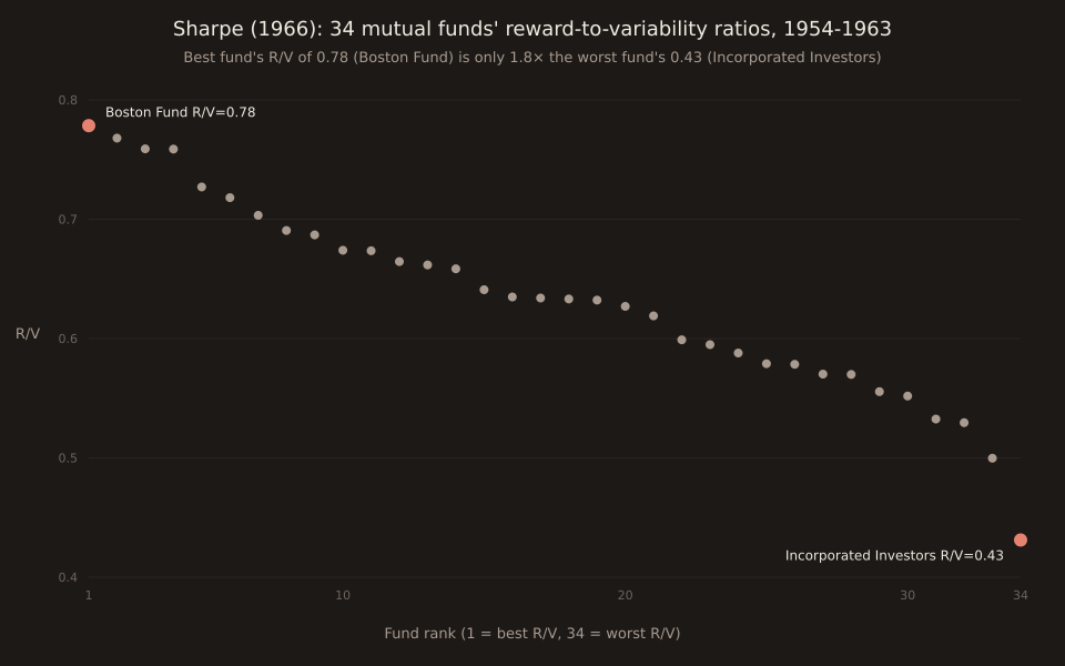
William F. Sharpe’s 1966 Journal of Business paper introduced the reward-to-variability ratio — what the industry now calls the Sharpe ratio — and applied it to 34 open-end mutual funds over the decade 1954-1963. The best fund’s R/V of 0.78 was only 1.8×the worst fund’s 0.43. Rank correlation between the R/V and the earlier Treynor Index across the same 34 funds: +0.974. Past-decade R/V had a +0.360 Spearman rank correlation with next-decade R/V — modest, but a full two standard errors above zero.
Yesterday’s Stats for Traders #8 introduced the Sharpe ratio as a modern trading tool — how to compute it, how to annualise it, what its assumptions violate on FX-event data. Today’s Stats #9 introduces the Sortino ratio as a downside-only variant of the same metric. Neither installment gave the ratio’s historical origin. This post is that origin: the 1966 paper where Sharpe first defined what he then called the R/V ratio, tested it on real mutual-fund data, and set the template for how the finance industry has thought about risk-adjusted performance ever since.
The paper in one paragraph
Sharpe extends Jack Treynor’s earlier 1965 Harvard Business Review article (which had proposed a beta-normalised performance metric). Sharpe’s modification: replace market-beta in the denominator with total standard deviation of annual return, which captures both systematic and idiosyncratic risk. He calls the result the reward-to-variability ratio (R/V) and defines it as:
R/V = (average annual return − pure interest rate) / variability Where "pure interest rate" = yield on a 10-year US Treasury. Sharpe uses 3.0% for 1954-1963 and 2.5% for 1944-1953.
Applied to a sample of 34 open-end mutual funds (data source: Arthur Weisenberger & Co.’s Investment Companies 1953, 1962, and 1964 editions), Sharpe finds R/V ratios spanning a surprisingly narrow range from 0.43 (Incorporated Investors) to 0.78 (Boston Fund). Only a 1.8× spread across the full sample of professional managers.
The R/V-vs-Treynor cross-check: +0.974
Sharpe explicitly wanted to know whether his new R/V ratio produced meaningfully different rankings from the Treynor Index it was extending. Spearman rank correlation across the 34 funds, same 1954-63 period: +0.974. Nearly identical rankings.
The mathematical intuition: when a fund’s return variance is dominated by market co-movement, total standard deviation is approximately proportional to market-beta. Dividing average excess return by total std or by beta then produces very similar rankings. Sharpe verifies this in Figure 3 of the paper: the median fund gets 90.33% of its return variance from co-movement with the Dow-Jones Industrial Average (average across 34 funds: 87.88%). At that level of market exposure, R/V and Treynor are effectively the same metric.
For modern strategies with low market-beta but high idiosyncratic variance — a hedge fund with market-neutral pairs trades, a systematic FX strategy like the ones this newsletter analyses — R/V and Treynor WOULD diverge. Sharpe’s ratio would still be defined and interpretable; Treynor’s ratio would break down (a beta near zero produces a divide-by-zero instability). That’s why the industry eventually converged on Sharpe’s formulation over Treynor’s.
The predictive test: past R/V modestly forecasts future R/V
Section IV re-computes R/V ratios for the same 34 funds over the prior decade (1944-1953) and checks whether past-decade rankings forecast future-decade rankings. Spearman rank correlation: +0.360. Standard error for the sample size (n=34): 0.174. So the observed correlation is about two standard errors above zero — statistically distinguishable from noise, but genuinely modest.
Sharpe’s own framing (paper page 126): “the relationship is far from perfect, [but] there is a general upward trend”. The practical takeaway is the origin of the “past performance does not guarantee future results” regulatory disclaimer: a fund’s historical R/V is some evidence about its future R/V, but not much. This finding preceded Jensen (1968), which is the paper cited in Fama (1970, Paper Trail #4) for evidence that mutual funds do not persistently beat the market net of costs.
Expenses matter: the −2.07 t-statistic
Section V regresses R/V ratios on prior-decade Treynor Index (as a control for “skill persistence”) and on the expense ratio and dividend ratio as of December 1953. The coefficient on expense ratio in the simplest single-variable specification: t = -2.07 — statistically significant at 5%, negative sign. Higher-expense funds systematically produced lower R/V ratios across the sample.
This is the empirical foundation John Bogle built Vanguard on in 1975, and the empirical foundation the modern indexing industry has scaled on: an active mutual fund charging 1.5%annual fees needs to persistently outperform a passive index by 1.5% just to break even, and the historical record from 1954 onwards suggests most funds don’t. Ties back to Paper Trail #7 (Barber & Odean 2000), which showed retail investors eating a similar 5-7 percentage points per year in trading costs against a market benchmark. Expense drag is the single most consistent finding across the risk-adjusted-performance literature from Sharpe 1966 forward.
What today’s Sharpe ratio inherits from the 1966 version
Practically everything. Yesterday’s Stats #8 used the formula (mean return − risk-free rate) / std— Sharpe’s 1966 R/V ratio verbatim. The four assumptions listed there (IID returns, normality, zero-cost execution, constant risk-free rate) are the same four assumptions Sharpe’s 1966 sample of buy-and-hold mutual funds approximately satisfied (annual buy-and-hold means IID year-over-year, no execution cost inside a fund’s pre-computed NAV, and the “pure interest rate” assumption Sharpe explicitly names on page 122). Today’s Sortino discussion is Frank Sortino’s 1980 refinement: replace the symmetric denominator with a downside-only version.
The one significant change since 1966: the industry now annualises. Sharpe worked with 10-year mean and std, so his R/V numbers are directly interpretable — the mean and std are already annualised because the underlying return series was annual returns. Modern hedge-fund reporting uses per-trade or per-daily Sharpe multiplied by sqrt(N per year). Yesterday’s Stats #8 walked through that annualisation.
Reading the paper today
The 1966 text is short (twenty pages, easy read), heavy on prose relative to modern JFE-style papers, and uses graphical arguments (Figures 1-6) that would today be flagged as under-formalised. But every core insight of modern risk-adjusted performance measurement is in the text: the reward-to-variability formula, the equivalence with Treynor under high market-beta, the modest predictive power of past performance, and the empirical dominance of expense ratios as a return-predictor. Sharpe won the 1990 Nobel Prize in Economics (shared with Markowitz and Miller) primarily for CAPM (a separate 1964 paper), but the 1966 mutual-fund paper is what put the R/V ratio into working circulation in the industry.
The paper is behind JSTOR’s paywall at jstor.org/stable/2351741. A course-materials mirror of the full PDF is available at UCLA’s statistics department (Christos course notes) at stat.ucla.edu (the source I read for this post).