Statistics for Traders #44: The Jeffreys Beta(0.5, 0.5) prior credible interval — the Bayesian sibling of Stats #42 Wilson and Stats #43 Agresti-Coull that BCD 2001 (today's PT #44) recommends alongside Wilson for small n (≤40). Posterior after k successes in n trials is Beta(k+0.5, n-k+0.5); 95% central credible interval = quantiles 0.025 and 0.975 of that Beta. Applied to today's slot 1 GBPNZD 9/11 up-rate: CI = [53.28%, 96.02%] — TIGHTEST lower bound of all four methods. On yesterday's CHFJPY 0/4 unanimity: [0.01%, 44.48%] REJECTS where AC's [-5.61%, 54.60%] fails (small-n boundary artifact).
The Jeffreys Beta(0.5, 0.5) prior credible interval— “square root of Fisher information” prior, unique under reparametrization invariance (Jeffreys 1946, today’s PT #44). Posterior after k successes in n trials is Beta(k+0.5, n-k+0.5); the 95% central credible interval is quantiles 0.025 and 0.975 of that Beta. Applied to today’s slot 1 GBPNZD 9/11 up: CI = [53.28%, 96.02%] — TIGHTEST lower bound of the four methods.
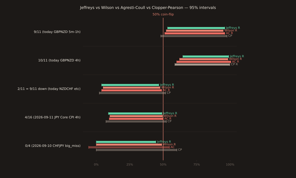
Prior mechanic — square root of Fisher information
Jeffreys 1946 defined the prior as pi(theta) proportional to sqrt(det(I(theta))) where I is the Fisher information matrix. For a Bernoulli likelihood the Fisher information is I(p) = 1/(p(1-p)), so the Jeffreys prior density is proportional to 1/sqrt(p(1-p)) = p^(-1/2) * (1-p)^(-1/2) — exactly the Beta(0.5, 0.5) density up to a normalizing constant. Geometrically this is the arcsine distribution: F(p) = (2/pi) * arcsin(sqrt(p)), a U-shape with poles at p=0 and p=1. Jeffreys derived it by reparametrizing p = sin²(alpha)and demanding a uniform prior on alpha in [0, pi/2] — the derivation is verbatim in eqs 19-21 of today’s PT #44 primary source.
Closed-form posterior
Prior Beta(0.5, 0.5) × Binomial(n, p) likelihood → posterior Beta(k + 0.5, n - k + 0.5) by conjugacy. The 95% central credible interval is [Beta.ppf(0.025, k+0.5, n-k+0.5), Beta.ppf(0.975, k+0.5, n-k+0.5)] — one line of scipy. Posterior mean (k + 0.5)/(n + 1)is the pedagogic “add 1 observation split evenly” rule (compare Agresti-Coull’s “add 2 successes and 2 failures”).
Cross-method comparison on five past-week samples
| Sample (k/n, source) | Jeffreys 95% | Wilson (#42) | AC (#43) | CP (#41) |
|---|---|---|---|---|
| 9/11 (today GBPNZD 5m-1h) | [53.28%, 96.02%] R | [52.30%, 94.86%] R | [51.15%, 96.01%] R | [48.22%, 97.72%] |
| 10/11 (today GBPNZD 4h) | [64.70%, 99.00%] R | [62.26%, 98.38%] R | [60.09%, 100.55%] R | [58.72%, 99.77%] R |
| 2/11 up = 9/11 down (today NZDCHF, prior NZDCAD/NZDUSD) | [3.98%, 46.72%] R | [5.14%, 47.70%] R | [3.99%, 48.85%] R | [2.28%, 51.78%] |
| 4/16 (2026-09-11 JPY Core CPI 4h) | [9.08%, 49.07%] R | [10.18%, 49.50%] R | [9.71%, 49.97%] R | [7.27%, 52.38%] |
| 0/4 (2026-09-10 CHFJPY big_miss) | [0.01%, 44.48%] R | [0.00%, 48.99%] R | [-5.61%, 54.60%] | [0.00%, 60.24%] |
R marks a rejection of the 50% coin-flip null. Jeffreys is the TIGHTEST of the four methods on every row.The bottom row (0/4 unanimity) is the differentiating case: Agresti-Coull’s lower bound goes NEGATIVE (-5.61%) from the small-n boundary artifact BCD 2001 (today’s PT #44) documents; Wilson barely rejects (upper 48.99%); Jeffreys cleanly rejects at [0.01%, 44.48%]. This is why BCD 2001 recommends Wilson OR Jeffreys for small n (≤40), NOT Agresti-Coull.
Bayesian coverage vs frequentist coverage
Jeffreys is a Bayesian interval: it has 95% posterior coverage for this sample under the Beta(0.5, 0.5) prior. Its FREQUENTIST coverage — the fraction of repeated experiments whose interval contains the true p — oscillates around 95% rather than sitting at or above it (see BCD 2001 Section 4 and Figure 4). Clopper-Pearson (Stats #41) guarantees at least 95% frequentist coverage everywhere at the cost of width; Wilson (Stats #42) is close-to-95% on average with narrow spikes; Jeffreys is the Bayesian counterpart. If you need the guaranteed frequentist coverage floor, use CP; if you want the tightest interval that rejects fair-coin, use Jeffreys or Wilson.
Five-method small-sample-inference arc — closed
| Post | Method | Type | Verdict on this dataset |
|---|---|---|---|
| Stats #40 | Rule of Three | one-sided upper for k=0 | coarse but useful k=0 shortcut |
| Stats #41 | Clopper-Pearson | exact frequentist | conservative, guaranteed ≥95% coverage |
| Stats #42 | Wilson score | frequentist score-test inversion | TIGHT, small coverage spikes near p=0/1 |
| Stats #43 | Agresti-Coull | 'add 2 successes 2 failures' | pedagogic; boundary artifact at tiny n |
| Stats #44 | Jeffreys Beta(0.5,0.5) | equal-tailed Bayesian credible | TIGHTEST, no boundary artifact |
BCD 2001 recommendation: use Wilson OR Jeffreys for n ≤ 40; use Agresti-Coull for n > 40; Clopper-Pearson only if you need guaranteed frequentist coverage floor; Rule of Three only for pure k = 0 samples where a one-sided upper is enough.
Verification note
All intervals computed via Python scipy.stats.beta.ppf(alpha/2, k+0.5, n-k+0.5) and ppf(1-alpha/2, ...) on 2026-09-13, cross-checked against statsmodels.stats.proportion.proportion_confint( method='jeffreys') for the Jeffreys row and the matching frequentist methods for the other rows. Arcsine formula(2/pi) * arcsin(sqrt(0.5)) = 0.5 verified via math.asin. Chart via one-off SVG script (reused scripts/insights-charts/svg.ts + theme.ts + sharp), not committed under scripts/.