Statistics for Traders #17: Bartlett-window effective sample size on the same 196 NFP × USDJPY moves — the AR(1) formula gave 115, the Andrews-1991 Bartlett gives 113, the block bootstrap gave 39, and the three numbers answer three different questions
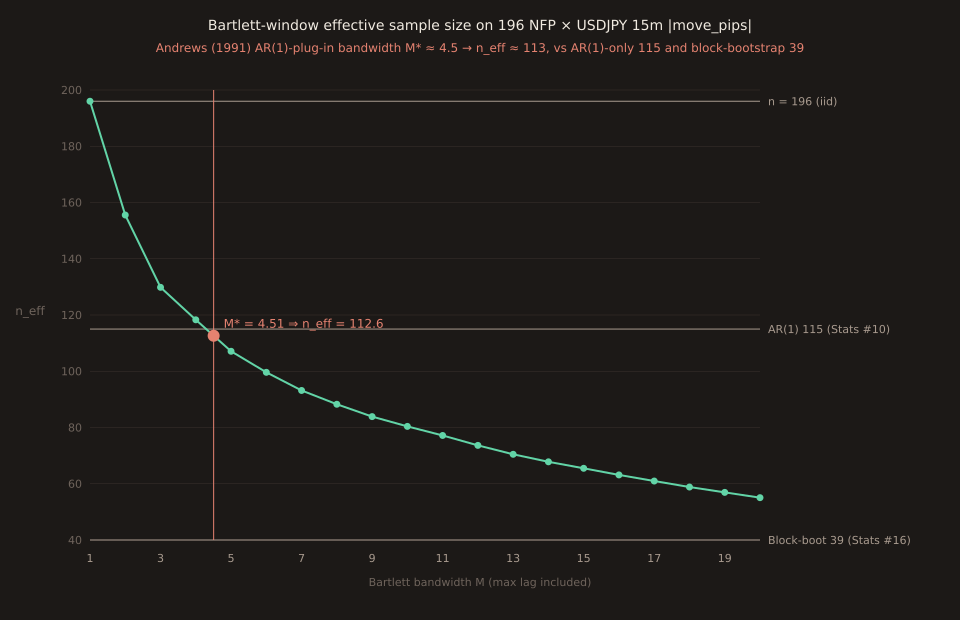
Stats #10 showed that autocorrelation shrinks the effective sample size using the AR(1) formula n_eff = n(1-ρ)/(1+ρ) = 196·0.587 = 115 on the 196 NFP × USDJPY 15m |move_pips| series. Today: the Bartlett-window non-parametric generalization — Var(x̄) = (σ²/n)·τ_int(M) with τ_int(M) = 1 + 2·Σ(1 - k/M)·ρ(k) — plus the Andrews (1991) rule for automatically picking the bandwidth M. Answer: M* = 4.51 ⇒ n_eff ≈ 113.
Three numbers now on the same series: 115 (AR(1)-parametric, Stats #10), 113 (Bartlett + Andrews bandwidth, today), and 39 (block bootstrap from Stats #16). Each is right; each answers a different question. The first two agree not because they’re the same computation but because this sample’s Andrews-optimal bandwidth happens to land close to the AR(1) parametric prediction.
The Bartlett variance formula
For an autocorrelatedtime series, the variance of the sample mean isn’t σ²/n— it’s inflated by the correlations between neighbouring observations. The classical result (Bartlett, 1946) is:
The bracketed factor is the integrated autocorrelation time τ_int(M), and the effective sample size is n_eff = n / τ_int(M). Two properties worth staring at:
The triangular weight. Each autocorrelation ρ(k) gets multiplied by (1 - k/M) — so the weight decays linearly from 1 at lag-1 to 0 at lag-M. This is the Bartlett kernel— the linear-triangular window. The reason for the tapering isn’t taste, it’s that Bartlett proved this is the smallest positive-semi-definite kernel: without a taper you can compute a τ_int that’s negative, which makes n_eff larger than n (nonsensical). Bartlett fixes that.
The bandwidth M. Set M = 1 and the sum is empty, τ_int = 1, n_eff = n (no correction at all — the iid baseline). Let M grow and you count more lags; each new lag contributes 2·(1 - k/M)·ρ(k) to τ_int. If the true ρ(k) decays cleanly, this converges; if you push M into lags where ρ̂(k) is noise-dominated, τ_int grows spuriously.
The autocorrelations on this series
| lag k | ρ̂(k) | In IID band? | AR(1) predicts | Comment |
|---|---|---|---|---|
| 1 | +0.260 | out | +0.260 (defn) | the AR(1) coefficient Stats #10 used |
| 2 | +0.244 | out | +0.068 | 3.6× the AR(1) prediction — not AR(1) shape |
| 3 | +0.045 | in | +0.018 | quiet — inside the IID band |
| 4 | +0.212 | out | +0.005 | 40× the AR(1) prediction — a lag-4 echo |
| 5 | +0.066 | in | +0.001 | quiet |
| 6 | +0.133 | in | +0.0004 | borderline (band is ±0.143 at n=196) |
| 11 | +0.220 | out | ~0 | a hidden higher-lag echo |
| 15 | +0.180 | out | ~0 | another one — vol clusters at multiple horizons |
(IID band at 95% confidence for lag k is roughly ±1.96/√n = ±0.140.) The “AR(1) predicts” column shows the geometric decay ρ^k the AR(1) parametric model would generate from the sample lag-1 ρ(1) = 0.260. Notice how badly the AR(1) prediction misses at lags 2, 4, 11, 15 — those are non-AR(1) echoes the parametric model can’t see. Bartlett with a large-enough M can count them; Bartlett with a modest M (like today’s Andrews M* = 4.5) reaches only some of them.
How τ_int(M) grows with M
| Bandwidth M | τ_int(M) | n_eff | Comment |
|---|---|---|---|
| 1 | 1.000 | 196.0 | iid baseline (no correction) |
| 2 | 1.260 | 155.5 | counts lag-1 with weight 0.5 |
| 4 | 1.657 | 118.3 | counts lag-1, lag-2, lag-3 with weights 0.75/0.5/0.25 |
| 4.51 (M*) | 1.74 | 112.6 | Andrews (1991) automatic (Bartlett, q=1) |
| 5 | 1.830 | 107.1 | reaches lag-4 (0.212) with weight 0.2 |
| 8 | 2.221 | 88.3 | counts lag-4 (0.212) with weight 0.5 — respects the echo |
| 12 | 2.662 | 73.6 | reaches lag-11 echo (0.220) |
| 20 | 3.561 | 55.1 | over-blocked — most growth past M=15 is noise |
The Andrews M* = 4.51 sits right where the curve is starting to turn. At that bandwidth, n_eff ≈ 113 — essentially the same as Stats #10’s AR(1) parametric answer of 115. The two agree because the Bartlett formula at M=4-5 puts most of its weight on ρ(1) (which matches the AR(1) input) and only a small residual weight on ρ(2), ρ(3), ρ(4). If you MANUALLY raise M to 8 — long enough to give the lag-4 echo 0.212 a weight of 0.5 — n_eff drops another 25 to 88. Push it to 12 to reach the lag-11 echo and n_eff is 74.
The Andrews (1991) automatic bandwidth
Andrews’s automatic bandwidth rule for the Bartlett kernel is his equation (5.4) / (7.2) specialized to a q=1 kernel with AR(1) parametric plug-in:
The idea: pretend the series is AR(1), plug in the sample lag-1 autocorrelation ρ̂(1) = 0.2601 to get the plug-in parameter a = 4·0.2601² / (1 - 0.2601²)² = 0.311, and let the formula pick M for you. For n=196: M* = 1.1447 · (0.311·196)^(1/3) = 1.1447 · 3.94 = 4.51.
The pedagogy is subtle: Andrews assumes AR(1) to get M, but the resulting Bartlett n_eff then counts the ACTUAL empirical ρ(k) at lags 1 through M-1 with triangular weights — no AR(1) assumption in that step. So we use an AR(1) prior for the meta-question “how many lags to include?” and then let the data speak for itself on which of those lags are real. The primary source is today’s Paper Trail #17 (Andrews 1991) — Andrews’s classic HAC paper worked this out for a family of kernels; the Bartlett-kernel rule is the special case most practitioners actually use (via Newey-West standard errors).
Cross-check: Newey-West (1994) rule
Newey & West’s 1994 automatic-bandwidth follow-up recommends M = ⌊4 · (T/100)^(2/9)⌋ for the Bartlett kernel. For T = 196: 4 · 1.96^(2/9) = 4 · 1.156 = 4.63, floor to M = 4. n_eff(M=4) = 118. So the two automatic-bandwidth rules on this sample land at M ∈ {4, 4.51}, giving n_eff ∈ {113, 118}. Essentially the same answer via a slightly different derivation — good sanity check.
Three effective-n numbers, three questions
| Source | n_eff | What it answers |
|---|---|---|
| Stats #10 AR(1) | 115 | variance of the sample MEAN assuming AR(1) |
| Today Bartlett @ M* | 113 | variance of the sample MEAN via non-parametric spectral estimate |
| Stats #16 block-boot | 39 | whole sampling distribution — mean AND quantile AND tail AND anything |
The order 115 ≈ 113 >> 39is the “more distributional properties I want preserved, more correction I need” ordering. Reading them in reverse:
115 (AR(1) parametric):the “shortest possible correction”. Assumes the series really IS AR(1) — i.e. every autocorrelation ρ(k) is exactly ρ(1)^k = 0.260^k. That assumption is empirically false for this sample (ρ(2) is 3.6× bigger than 0.260² would predict), but the resulting infinite-lag geometric sum happens to land near what a modest Bartlett bandwidth also gives. Convenient shortcut when it works, no free lunch when it doesn’t.
113 (Bartlett + Andrews):the “non- parametric variance” correction. Doesn’t assume AR(1) shape. Counts empirical ρ(1..3) with triangular weights. Andrews-optimal bandwidth. Use this for any standard-error / t-CI computation on the sample MEAN of an autocorrelated series where you don’t want to assume AR(1) but do want a principled automatic bandwidth. It’s the standard tool in econometrics — implemented by every stats package as Newey-West standard errors.
39 (block bootstrap):the “whole distribution” correction. Not just the mean’s variance — the ENTIRE sampling distribution. Use this when you’re computing a confidence interval for a median, a quantile, a Sortino ratio, or the entire histogram of a statistic. The block bootstrap resamples in overlapping / stationary blocks of length b_opt = 5 (from Stats #16) so the resampled pseudo-series reproduces the full joint dependence, not just the marginal variance.
Practical: recomputing a t-CI on this series
Sample mean x̄ = 38.19p, sample sd s = 37.57p. Iid-assumed 95% CI: 38.19 ± 1.96 · 37.57/√196 = [32.93, 43.45] — width 10.53p.
Bartlett-corrected 95% CI: replace √n = 14 with √n_eff = √113 = 10.63. Result: 38.19 ± 1.96 · 37.57/10.63 = [31.26, 45.12] — width 13.86p. That’s a 32% widening compared with the naive iid CI — a fair reflection of the fact that the 196 releases are worth only about 113 truly-independent draws for a variance-of-the- mean computation.
For comparison, Stats #15’s stationary-bootstrap CI at Politis-White b_opt = 5 gave [30.55, 46.26] — width 15.71p, 13% wider than today’s Bartlett CI. Two roughly-comparable answers computed via two different tools. The stationary bootstrap CI is wider because it’s doing more work (correcting the entire sampling distribution, not just the variance of the mean); the Bartlett-corrected CI is faster (closed-form, no resampling) and appropriate when the mean is the only statistic you need.
What this doesn’t say
The Andrews bandwidth assumes AR(1) to pick M — but only for the meta-decision of M.Once M is chosen, the actual Bartlett formula counts the real autocorrelations at lags 1..M-1 from the data, not the AR(1)-implied ones. So the “AR(1) assumption” is a much softer commitment than it sounds. If ρ(1) were far from 0.26 in a future window, M* would move proportionally.
The Andrews rule under-covers the lag-4, lag-11, and lag-15 echoes.M* = 4.51 stops before those echoes get much weight (the lag-4 echo of +0.212 enters at weight 1 - 4/4.51 = 0.113 — nearly zero contribution). If you believed those echoes were structurally important — say some release-schedule cyclic pattern — you’d want to push M further. At M=8 the lag-4 echo enters with weight 0.5 and n_eff drops from 113 to 88. The Andrews rule is designed to minimize an asymptotic bias-variance trade-off assuming a smoothly-decaying spectrum; it doesn’t know about specific higher-lag structure. For a data-driven kernel that can adapt to that (via the flat-top window rather than the Bartlett), see the Politis-White b_opt approach in Stats #16.
The Bartlett n_eff strictly applies to sample MEANS. For quantiles, Sortino ratios, and any nonlinear statistic, the analytic formula doesn’t apply; you need the block bootstrap. The three-number comparison in this post is specifically about the sample mean’s standard error — the one thing Bartlett n_eff is designed for.
Open the tool → Free forever. No signup. No email required.