Statistics for Traders #9: Sortino ratio via the CAD Unemployment × USDCAD big-beat bucket — a Sortino of 4.79 vs a Sharpe of 0.98, and why the gap tells you the loss distribution is asymmetric
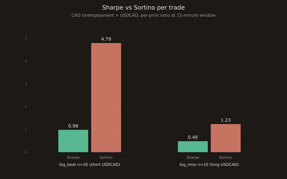
The 26 big-beat CAD Unemployment prints on USDCAD produce a per-trade Sharpe ratio of 0.98 for a short-USDCAD strategy — respectable but not extraordinary. The Sortino ratio on the same 26 trades is 4.79. That’s not a computational quirk. 22 of the 26 trades won, and 3 of the 4 losers were tiny (-3.2, -3.5, -9.0 pips). Only one trade — 2017-08-04 at -35.1p — was a meaningful loss. Sortino divides mean return by the RMS of downside returns and finds almost nothing to divide by. That’s the point.
Today’s slot-1 post established that CAD Unemployment on USDCAD walks monotonically across the five surprise buckets. The big_beat bucket — n=26, median 15-minute move −39.3p, pct-up 15% — is the sample this installment works through. Yesterday’s Stats for Traders #8 introduced Sharpe as “mean over standard deviation” and flagged that a symmetric denominator under-weights strategies with asymmetric loss distributions. Sortino is that correction, and the CAD Unemployment × USDCAD big_beat bucket is a beautifully clean worked example of when Sortino and Sharpe diverge.
The formula
Sortino = mean return / downside deviation. Four steps:
step 1 mean = sum(returns) / n step 2 for each return r_i, compute downside_i = max(0, MAR - r_i) MAR ("minimum acceptable return") is usually 0. When MAR = 0, downside_i = max(0, -r_i) — the loss magnitude for losing trades, 0 for winning trades. step 3 downside_dev = sqrt( sum(downside_i²) / n ) ↑ divide by full n, not loser count step 4 Sortino = mean / downside_dev
The one thing to know about the denominator: divide the sum of squared downside returns by the full sample size n, NOT by the count of losing trades. This is the convention in Bacon’s Practical Portfolio Performance Measurement and Attribution (2013) and in most institutional performance software. Winning trades contribute 0 to the sum but still count toward n, so the denominator gets diluted by winners. The alternative (divide by loser count) inflates Sortino to implausible values on high-win-rate strategies.
Worked example: CAD Unemployment × USDCAD big_beat, all 26 prints
The strategy: short USDCAD 15 minutes before a big_beat CAD Unemployment print, cover 15 minutes after. Per-trade PnL = -move_pips. A big_beat print for unemployment is a print where the unemployment rate came in LOWER than consensus (a favourable surprise for CAD), so the base rate is CAD strong → USDCAD down → our short wins.
n = 26 sum(PnL) = +892.5 pips mean = +34.33 pips sample variance (n-1 denom) = 1229.6 sample sd = 35.07 pips Sharpe (per-trade, r_f=0) = 34.33 / 35.07 = 0.979 Losing trades (move_pips > 0): 4 of 26 2017-08-04 cons=6.5 act=6.3 move=+35.10 → PnL = -35.10p 2010-12-03 cons=7.9 act=7.6 move= +9.00 → PnL = -9.00p 2020-05-08 cons=18.0 act=13.0 move= +3.50 → PnL = -3.50p 2026-02-06 cons=6.8 act=6.5 move= +3.20 → PnL = -3.20p Sum of squared losses = 35.1² + 9² + 3.5² + 3.2² = 1232.01 + 81 + 12.25 + 10.24 = 1335.50 Downside dev (Bacon, n=26) = sqrt(1335.50 / 26) = sqrt(51.365) = 7.167 pips Sortino (per-trade, MAR=0) = 34.33 / 7.17 = 4.790
Sharpe 0.98, Sortino 4.79. Sortino is 4.9× the Sharpe.
Why the ratio Sortino/Sharpe is diagnostic
For a perfectly symmetric distribution — the normal or any distribution where upside and downside contribute equally to total variance — Sortino equals Sharpe × sqrt(2). That’s a mathematical identity, not an empirical rule. sqrt(2) ≈ 1.414. So the ratio Sortino/Sharpe = 1.414 is the symmetric baseline. Any observed ratio above that means the empirical loss distribution is smaller or rarer than a symmetric distribution would predict.
On the big_beat bucket: Sortino/Sharpe = 4.79 / 0.98 = 4.89. That’s 3.5× the symmetric baseline. Very asymmetric — the strategy loses infrequently, and when it loses, loses small. On the big_miss bucket (long-USDCAD, n=10 with 3 losers): Sortino/Sharpe = 1.23 / 0.48 = 2.56, about 1.8× the baseline — noticeably asymmetric but nowhere near as extreme.
In practical terms: the big_beat bucket has a much better risk-reward tail shape than the big_miss bucket does, even though the Sharpes are only 2× apart. The Sortino gap widens that comparison substantially — 4.79 vs 1.23 is a 4× ratio.
Where Sortino misleads
Sortino is brittle when losers are rare. The big_beat bucket has 4 losing trades in a sample of 26. Adding one more losing trade — say, at -50 pips (larger than any historical loser) — would recompute as:
new sum of squared losses = 1335.50 + 50² = 3835.50 new downside dev = sqrt(3835.50 / 27) = 11.92p new mean (approx) = (892.5 - 50) / 27 = 31.2p new Sortino = 31.2 / 11.92 = 2.62
A single new loser at -50 pips would drop the Sortino from 4.79 to 2.62 — almost half. Same distribution, one more data point, wildly different summary statistic. This is the identical fat-tail problem Stats #6 (kurtosis) established for raw return distributions, applied to the Sortino estimator itself. Rule of thumb: if the loser count is below 20, treat the Sortino as informative-but-noisy. Below 10 — big_miss with 3 losers is well below — treat it as directional only.
Sortino is not annualized here. The 4.79 is per-trade, not annualized. Both CAD Unemployment big-beat prints and big-miss prints fire only a few times per year (roughly 2-3 big_beat and 1-2 big_miss annually on this event×instrument), so annualized Sortino for either strategy = per-trade Sortino × sqrt(2 or 3). For big_beat: sqrt(2.5) × 4.79 ≈ 7.6 annualized. Still very high. Still driven by 4 losing trades in the historical record. Still brittle to the next big loser.
What’s next in the series
Sortino is the first genuine risk-adjusted-return metric this series has introduced that isn’t symmetric in its treatment of upside and downside. Two natural follow-ups from the ledger’s queue: the information ratio(Sharpe against a benchmark instead of the risk-free rate — a fair-comparison metric when you’re trying to say your strategy beats a passive long-USDCAD baseline, rather than just beats zero) and bootstrap resamplingfor tail-bucket confidence intervals (flagged as the tool of choice back in Stats #7 for the same small-n problem that makes Sortino brittle here). Also on deck: correlation vs causation (a worked FX example) and autocorrelation (why 20 back-to-back candles don’t count as 20 observations, and how that inflates the effective variance in the Sortino denominator).
Open the tool → Free forever. No signup. No email required.