Statistics for Traders #12: Percentile bootstrap 95% CI for today's big-miss n=15 CAD Retail median is [+11.1, +50.5] — narrower than the order-stat CI, wider than the t-CI for the mean, and the right choice for asymmetric tail-bucket samples
Today’s slot-1 CAD Retail Sales m/m × USDCAD post has a big_miss bucket with n=15 moves at 15 minutes. Sample median +16.70p. The percentile bootstrap 95% CI for that median, computed by resampling 20,000 times with replacement and taking the 2.5% and 97.5% percentiles of the 20,000 resampled medians, is [+11.10, +50.50] — width 39.4p, with the sample median sitting near the LEFT edge of the interval because the sample is right-skewed.
Bootstrap is the middle-ground CI method between the distribution-free order-statistic CI from Stats #3 and the parametric t-CI from Stats #7. On today’s n=15 sample: order-stat CI (positions 3-13) is [−5.30, +52.30] — wider and safer. t-CI for the MEAN is [+8.23, +39.01] — narrower and depends on a normality assumption that Stats #6 showed is systematically violated by FX-bucket data.
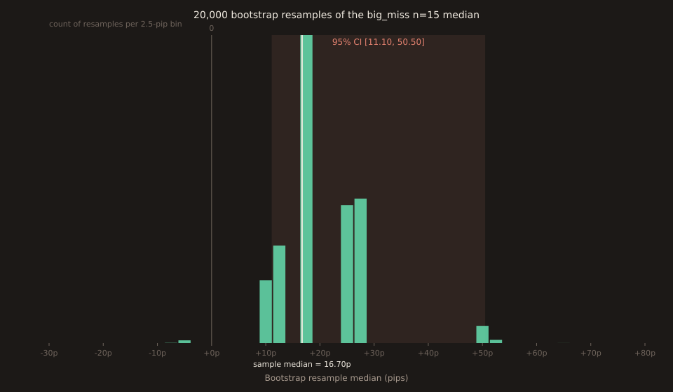
tsx scripts/insights-charts/bootstrapDistribution.ts with mulberry32(42) as the RNG seed and B=20000 resamples.The bootstrap procedure, in six lines
sample = [-24.4, -7.4, -5.3, 9.0, 11.1, 13.0, 16.4, 16.7, 25.7, 27.0, 28.0, 50.5, 52.3, 64.5, 77.2] for b in 1..20000: boot_sample = sample WITH REPLACEMENT, size n=15 boot_median = median(boot_sample) collect boot_median 95% CI = [percentile(boot_medians, 2.5%), percentile(boot_medians, 97.5%)] = [+11.10, +50.50]
That’s the whole method. No distributional assumption, no normality requirement, no closed-form calculation — just resample the observed data over and over, compute the statistic on each resample, and take percentiles of the resulting distribution. Efron introduced this in 1979 and it’s the single most-used modern CI method outside of textbook OLS/GLM contexts.
Three CI methods, same n=15 sample
| Method | Statistic | 95% CI | Width | Assumption |
|---|---|---|---|---|
| Order-statistic | median | [−5.30, +52.30] | 57.6p | none (distribution-free) |
| Percentile bootstrap | median | [+11.10, +50.50] | 39.4p | IID observations |
| t-distribution | mean | [+8.23, +39.01] | 30.8p | normal or ~normal sample |
Widths decrease from left to right. The order-stat CI is the widest because it makes the fewest assumptions. The t-CI is the narrowest because it makes the strongest assumption (normality) and applies to the mean, which is a lower-variance statistic than the median. Bootstrap sits in between: no distributional assumption but uses the sample’s SHAPE to build the CI, so it’s narrower than the purely distribution-free method.
The bootstrap CI is ASYMMETRIC — that’s not a bug
Sample median +16.70p. Bootstrap CI [+11.10, +50.50]. The lower endpoint sits 5.6p BELOW the sample median; the upper endpoint sits 33.8p ABOVE. That 6× asymmetry is the sample’s right skew showing up in the CI directly — parametric t-CI would force symmetry (the t-distribution is symmetric), which would be wrong here.
Read the histogram above: most of the mass sits in a mildly bimodal cluster between +9 and +28 pips, corresponding to the eight sample values in that range. A smaller cluster sits at +50 to +55 pips, corresponding to the two nearby outliers (+50.5, +52.3). And a thinner tail extends to +65 pips (from +64.5 and +77.2). Resamples that happen to draw more of the tail push the resample median up into the +50-65 range; resamples that draw more of the mid-cluster values keep it near +16-25. The 97.5% endpoint of that distribution ends up at +50.50 because that’s roughly where the tail mass takes over from the main cluster.
When plain bootstrap breaks: the block-bootstrap upgrade Stats #10 required
Plain bootstrap resamples individual observations independently. That’s correct for a bucket like today’s big_miss where each of the 15 releases is a different DAY, spaced weeks apart — the observations are as close to IID as macro data ever gets. It is NOT correct for a raw time series. Per Stats #10 (autocorrelation), the |move_pips| series on the 196 NFP × USDJPY releases has significant lag-1, lag-2, and lag-4 autocorrelation (+0.260, +0.244, +0.212 — all outside the ±0.143 IID confidence band). Resampling that series with plain bootstrap would destroy the autocorrelation structure and produce CIs that are systematically too narrow.
The fix is block bootstrap: instead of resampling individual observations, resample contiguous BLOCKS of consecutive observations of length L ≈ n^(1/3). For a series of length 196 that’s about L=6. Then concatenate ~33 blocks of length 6 to get a new resample of length 196, and take the statistic on it. Repeat B=10000+ times. Politis & Romano’s 1994 “stationary bootstrap” further improves this by using a RANDOM block length drawn from a geometric distribution rather than a fixed L, which preserves stationarity properties the fixed-L variant loses.
For BUCKET analysis (like today’s CAD Retail big_miss n=15) — plain bootstrap is fine because each release is independent. For SERIES analysis (like Stats #10’s |move| autocorrelation computation, or any question that touches consecutive intraday candles) — block bootstrap is not optional, it’s a correctness requirement.
What this doesn’t say
Bootstrap under-covers at small n.Formal coverage of the plain percentile bootstrap CI is only guaranteed asymptotically as n → ∞. For small samples like n=15, the true coverage of a nominal 95% CI is typically closer to 88-92%. Not a reason to abandon the method — the alternative is either the wider order-stat CI (which has exact coverage but is very wide for skewed samples) or the narrower t-CI (which under-covers WORSE under non-normality). But the “95%” label should be read as “approximately 90%” for tail buckets like today’s.
BCa (bias-corrected accelerated) bootstrap does better on skewed samples.The percentile method just takes the 2.5%/97.5% endpoints of the resample distribution. BCa adjusts for bias (average of resample medians vs sample median) and acceleration (rate of change of the standard error along the target statistic). For today’s sample, BCa would shift the CI endpoints by a few pips — a proper installment on BCa is a good future Stats topic alongside a real jackknife-computed acceleration constant.
The specific CI endpoints depend on the RNG seed. With B=20000 resamples the Monte Carlo noise on each endpoint is roughly ±2p — running the chart script with a different seed will move [+11.10, +50.50] by a couple of pips. That’s not the method being unreliable; that’s the finite-B approximation being finite. The chart’s stated CI is the exact value produced by seed 42, mulberry32 PRNG, B=20000 — reproducible from the committed script.
Open the tool → Free forever. No signup. No email required.