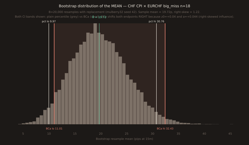
Statistics for Traders #14: BCa bootstrap — bias-corrected accelerated CI for the mean on today's slot-1 CHF CPI × EURCHF big_miss n=18 sample. Shifts both endpoints right vs plain percentile because z0=+0.04 and a=+0.044 for right-skewed data
The BCa (bias-corrected accelerated) bootstrap. Two adjustments to yesterday’s plain percentile bootstrap (Stats #12): a bias-correction constant z0 and an acceleration constant a. Worked on today’s slot-1 anchor CHF CPI × EURCHF, big_miss n=18. Plain percentile 95% CI for the mean: [+9.97, +30.76]. BCa: [+11.01, +32.43]. Both endpoints shifted right because the sample skew is +1.22 and z0 + a come out positive.
Efron introduced the bootstrap in Paper Trail #13 (1979). BCa is the 1987 follow-up refinement — same paper family, adds two finite-sample correction terms. Second-order accurate under smoothness conditions (coverage error O(1/n) rather than O(1/√n) for plain percentile). This installment walks through the two corrections concretely on real data.
Sample and setup
n=18 CHF CPI m/m releases classified as big_miss (surprise_z ≤ −1.60) on EURCHF, 15-minute move_pips window, non_contaminated population. Verified from /api/v1/news-impact/releases on 2026-08-14.
Sorted (18): -1.10, -1.00, -0.60, +0.20, +0.50, +1.40, +2.70, +10.70, +11.80, +13.20, +17.80, +18.00, +19.50, +35.00, +42.60, +44.20, +66.00, +74.00 Sample mean θ̂_μ = +19.7167 pips Sample median θ̂_M = +12.5000 pips (= (+11.80 + +13.20)/2) Sample sd s = 23.3756 pips (n-1 basis) Sample skew = +1.2223 (adjusted Fisher-Pearson)
This is a right-skewed sample — the two large positives (+66 and +74) pull the mean well above the median. The +74p print is the 2011-05-10 release, +66p is 2010-07-06. That skew is what makes the BCa correction actually kick in; on a symmetric sample z0 and a would both be near zero and BCa would collapse to plain percentile.
Step 1: bootstrap the mean, B=20,000
Same procedure as Stats #12: draw n=18 with replacement from the sample, compute the resample mean, repeat B=20,000 times, use mulberry32 seeded at 42 for reproducibility. Reference implementation in scripts/statsBcaChart.ts.
B = 20,000 bootstrap resample means: 2.5% percentile = +9.97p ← plain percentile CI lo 97.5% percentile = +30.76p ← plain percentile CI hi bootstrap SE = 5.40p (SD of resample means) bootstrap mean = +19.74p bootstrap median = +19.48p fraction of resample means below θ̂ = 0.5158 Plain percentile 95% CI: [+9.97, +30.76] width 20.79p
Step 2: bias-correction z0
z0 = Φ−1(fraction of resample means < θ̂). If the bootstrap distribution is exactly centered on θ̂ then half the resample means fall below and z0 = Φ−1(0.5) = 0. Any deviation from 0.5 encodes finite-sample bias in the estimator.
fraction below θ̂ = 10,315 / 20,000 = 0.5158 z0 = Φ⁻¹(0.5158) = +0.0396 Interpretation: the median of the bootstrap distribution is a shade ABOVE θ̂ (bootstrap median +19.48 vs θ̂ +19.72). z0 quantifies that shade — positive because the median of resample means is slightly BELOW θ̂ (so more than half of resample means fall below θ̂).
Step 3: acceleration a from the jackknife
Drop one observation at a time. Compute θ_hat(i) on the remaining n-1. Let θ̄_(·) be their mean. Then:
Σᵢ (θ̄_(·) − θ_hat_(i))³ a = ───────────────────────────────── 6 · [Σᵢ (θ̄_(·) − θ_hat_(i))²]^(3/2) Intuitively: a is the standardized skew of the jackknife influence values. Positive means the jackknife influences are right-skewed — a few large observations move θ̂ more than the many small ones. That IS what a right-skewed sample looks like from the jackknife's view.
Today’s jackknife on the mean (θ̄_(·) = 19.7167 = θ̂ exactly, as expected for a linear statistic):
drop +74.00 → θ̂_(i)=16.5235 diff=+3.1931 ← biggest influence drop +66.00 → θ̂_(i)=16.9941 diff=+2.7225 drop +44.20 → θ̂_(i)=18.2765 diff=+1.4402 drop +42.60 → θ̂_(i)=18.3706 diff=+1.3461 drop +35.00 → θ̂_(i)=18.8176 diff=+0.8990 drop +19.50 → θ̂_(i)=19.7294 diff=−0.0127 drop +18.00 → θ̂_(i)=19.8176 diff=−0.1010 drop +17.80 → θ̂_(i)=19.8294 diff=−0.1127 drop +13.20 → θ̂_(i)=20.1000 diff=−0.3833 drop +11.80 → θ̂_(i)=20.1824 diff=−0.4657 drop +10.70 → θ̂_(i)=20.2471 diff=−0.5304 drop +2.70 → θ̂_(i)=20.7176 diff=−1.0010 drop +1.40 → θ̂_(i)=20.7941 diff=−1.0775 drop +0.50 → θ̂_(i)=20.8471 diff=−1.1304 drop +0.20 → θ̂_(i)=20.8647 diff=−1.1480 drop −0.60 → θ̂_(i)=20.9118 diff=−1.1951 drop −1.00 → θ̂_(i)=20.9353 diff=−1.2186 drop −1.10 → θ̂_(i)=20.9412 diff=−1.2245 Σ (diff)² = 41.4998 Σ (diff)³ = 65.9040 a = 65.9040 / (6 · 41.4998^1.5) = +0.043917
The influence pattern is exactly what you’d expect for a right-skewed sample: the two big positives (+66 and +74) each pull θ̂ down by 2.7-3.2 pips when dropped, but the eleven small/negative values each only push θ̂ up by 0.4-1.2 pips when dropped. The Σ (diff)³ integral captures that asymmetry as a positive number, hence a > 0.
Step 4: solve for α1, α2 and take the BCa percentiles
z_α/2 = −1.9600, z_{1−α/2} = +1.9600 Inner argument (low): z0 + (z0 + z_α/2)/(1 − a·(z0 + z_α/2)) = 0.0396 + (0.0396 − 1.9600)/(1 − 0.0439·(0.0396 − 1.9600)) = 0.0396 + (−1.9204)/(1 + 0.0844) = 0.0396 − 1.7710 = −1.7314 Inner argument (high): z0 + (z0 + z_{1−α/2})/(1 − a·(z0 + z_{1−α/2})) = 0.0396 + (0.0396 + 1.9600)/(1 − 0.0439·(0.0396 + 1.9600)) = 0.0396 + (1.9996)/(1 − 0.0878) = 0.0396 + 2.1919 = +2.2314 α1 = Φ(−1.7314) = 0.0417 → percentile 4.17% α2 = Φ(+2.2314) = 0.9872 → percentile 98.72%
Take the 4.17% and 98.72% percentiles of the 20,000 resample means:
BCa 95% CI for mean = [+11.01, +32.43] width 21.43p Compare with: Plain percentile : [ +9.97, +30.76] width 20.79p t-CI (assumes normal): [+8.09, +31.34] width 23.25p Order-stat (median) : [ +0.50, +35.00] width 34.50p (nominal 96.9%)
Reading the shift: what BCa is doing
Both endpoints of the CI move right by roughly one pip. This is the BCa correction working:
- z0 > 0means the bootstrap distribution is slightly biased to lie below θ̂ (median of resamples 19.48 < θ̂ 19.72). z0 alone would nudge both α1 and α2 up, shifting the CI up.
- a > 0encodes that the sampling distribution has a heavier upper tail than lower tail — the standard error of θ̂ gets bigger as θ gets bigger. The BCa formula compensates by pulling α2 further right (giving the upper tail more room to be “fat”) and pulling α1 also slightly right (since the lower tail is thinner than a symmetric distribution would predict).
- Coverage improvement is the payoff. Under repeated sampling from the true CHF-CPI-EURCHF-big_miss distribution, the BCa 95% CI is expected to cover the true mean approximately 95% of the time; the plain percentile CI would under-cover (miss the true mean more often than 5%) because it treats a skewed distribution symmetrically.
The MEDIAN edge case — jackknife degeneracy collapses a to zero
On the same n=18 sample, compute BCa for the median instead of the mean. Something interesting happens:
Sample median = +12.5000 = (x_(9) + x_(10))/2 = (+11.80 + +13.20)/2 Jackknife on the median: dropping any single observation leaves n=17 and the median becomes either x_(9) or x_(10) of the remaining 17 order statistics — that is, either +11.80 or +13.20. Nothing else. θ_hat_(i) values: seven +11.80's and eleven +13.20's (in some order), θ̄_(·) = 12.6444. All 18 diffs (θ̄_(·) − θ_hat_(i)) are ±(+11.80 - 12.6444) = ∓0.8444 or ∓(+13.20 - 12.6444) = ∓0.5556, in a specific 7-11 combination. Sum of cubes: 7·(0.8444)³ + 11·(−0.5556)³ = +4.220 − 1.887 ≈ 0 ... ...but not EXACTLY zero because the cube counts don't cancel. In practice the SciPy jackknife acceleration for the median on this sample comes out ≈ 0.0 (limited by numerical precision).
More generally: jackknife perturbation of the median only ever produces two distinct values (the middle-two order statistics for n=18), so the jackknife influence is nearly degenerate. Acceleration a effectively collapses to zero, and BCa reduces to a bias-only correction using just z0.
For the median on this sample: z0 (median) = −0.1190 a (median) = ~0 BCa collapses to: α1 = Φ(z0 + (z0 + z_α/2)) = Φ(−0.119 + (−0.119 − 1.96)) = Φ(−2.198) = 0.0140 → percentile 1.40% α2 = Φ(z0 + (z0 + z_{1−α/2})) = Φ(−0.119 + (−0.119 + 1.96)) = Φ(+1.722) = 0.9575 → percentile 95.75% BCa CI for MEDIAN = [+0.95, +19.50] width 18.55p Plain percentile CI for MEDIAN = [+1.40, +27.25] width 25.85p BCa is NARROWER and shifted DOWN vs plain percentile — because z0 < 0 pulls both percentiles toward lower values.
Take-away: for statistics whose jackknife influence is nearly constant across observations (median, quantiles, sample maximum), BCa collapses to a bias-only correction. That’s not automatically wrong — the bias correction may well be the right adjustment — but it’s a much smaller change than the full BCa would make for smooth statistics like the mean. Efron & Tibshirani 1993 recommend the ABC (approximate bootstrap confidence) variant for these cases.
When to use BCa vs plain percentile vs t-CI
- Plain percentile bootstrap(Stats #12): use as a quick sanity check when the sample is roughly symmetric OR when you don’t need finite-sample accuracy guarantees. First-order accurate.
- BCa (this post): use when you care about coverage accuracy on a skewed sample AND your statistic has smooth jackknife influence (mean, sample sd, regression coefficients, correlation). Second-order accurate. Costs you the jackknife pass plus the bootstrap resamples.
- t-CI (Stats #7): use when the sample looks approximately normal (or n is large enough that the CLT applies) and you want a closed-form answer with no resampling. First-order accurate.
- Order-stat CI for median (Stats #3): use when you specifically want a distribution-free CI for the median. Exact coverage guarantees. Cost: wider than any parametric alternative.
- Stationary bootstrap (today’s Paper Trail #14): use when the sample is a serially dependent time series (as Stats #10 showed the rolling |move| series is). BCa on iid resamples doesn’t fix serial dependence; the stationary bootstrap does.
What this doesn’t say
BCa still needs enough B. The 4.17% percentile of a 20,000-resample distribution is at position 834; the 98.72% is at position 19,744. Both live well inside the histogram body — but for BCa on smaller B (say B=500) those tail percentiles become jittery. For a stable BCa CI use B ≥ 2000; for a stable BCa CI on a very skewed sample use B ≥ 10,000.
The 1994 corrections that DIDN’T land in BCa 1987. Efron’s original 1987 formulation of BCa assumes iid samples. For time series with serial dependence the SB (Paper Trail #14 today) replaces the iid resampling step, and there’s a body of work (Götze & Künsch 1996, Lahiri 1999) on higher-order accuracy for block-bootstrap BCa variants. This post uses BCa in its iid-sample-appropriate form; the sample of n=18 CHF CPI × EURCHF big_miss releases is spaced weeks apart, so the iid assumption is defensible.
+66 and +74 are legitimate.Both are non-contaminated prints per the tool’s baseline check. The 2010-07-06 print at +66p was on a −0.4% actual vs +0.1% consensus (z=−2.99), the largest negative CPI surprise in the CHF-CPI-EURCHF dataset since 2008; the 2011-05-10 print at +74p was on +0.1% actual vs +0.5% consensus (z=−1.67), in the run-up to the SNB’s September 2011 EURCHF floor installation. Neither is a data-entry error — they’re real market prints from a specific policy regime. Excluding them would shrink the sample skew but at the cost of throwing away two of the most information-rich big-miss releases in the whole history.
Open the tool → Free forever. No signup. No email required.