What's the empirical result behind that aphorism?

Cochrane's Table 2 reports 15-year long-run regression coefficients on dividend yield for the CRSP value-weighted market ex T-bill, 1947-2009 annual data, via the Campbell-Shiller (1988) present-value identity. Direct method (15-year ex-post returns): β(returns) = 1.01, β(dividends) = -0.11, β(dividend yield) = -0.11. VAR-implied at 15 years: β(returns) = 1.05, β(dividends) = 0.27, β(dividend yield) = 0.22. VAR infinite horizon: β(returns) = 1.35, β(dividends) = 0.35, β(dividend yield) = 0.00. In the 1970s the expectation was β(returns) = 0, β(dividends) = 1 — high P/D ratios reflected optimism about future dividend growth. The direct measurement flipped the story entirely: high P/D ratios entirely forecast LOW future returns, with no measurable dividend-growth-forecasting content.

The 1-year vs 5-year DP regression numbers?

Cochrane's Table 1 (§ 2.1): 1-year regression of returns on dividend yield gives β = 3.8 (t = 2.6, R² = 0.09) — modest R², what a naive reader would call unimportant. 5-year regression via Hansen-Hodrick (1983) correction: β = 20.6 (t = 3.4, R² = 0.28). The economic significance is much bigger than R² suggests: a 1-percentage-point increase in dividend yield forecasts nearly 4 percentage points MORE return over the next year — which is the same order of magnitude as the entire equity premium. Cochrane's § 2.1 aside: 'R² is a poor measure of economic significance in this context. The economic question is How much do expected returns vary over time? There will always be lots of unforecastable return movement.'

'Zoo of new factors' — what does he mean?

From § 3 onwards, Cochrane inventories the empirical factor literature that ballooned between the 1970s and 2011: CAPM (Sharpe 1964, Lintner 1965) was expected to explain the cross-section of expected returns. Instead, Fama-French 3-factor (1993 — PT #8), Carhart 4-factor (1997 — PT #11), Fama-French 5-factor (2015 — PT #22, published 4 years AFTER this Cochrane paper), Novy-Marx profitability (2013 — PT #24), Asness-Moskowitz-Pedersen value-momentum (2013 — PT #23), plus dozens of others (accruals, PEAD, investment, quality, low-vol, betting-against-beta, quality-minus-junk) each demand a spot as a 'factor'. Cochrane's critique: with roughly 300 published factors as of 2011 (Harvey-Liu-Zhu 2016 later counts 316), most are almost certainly artifacts of multiple-testing bias and data mining, not real risk premia.

How does this connect to Fama 1970 (Paper Trail #4)?

PT #4 Fama 1970 argued (Cochrane § 1 verbatim): '40 years ago, Gene Fama (1970) argued that the expected part, testing market efficiency, provided the framework for organizing asset-pricing research in that era.' Cochrane 2011 § 1: 'I argue that the discounted part better organizes our research today.' The paper is explicitly framed as the second-half-of-Fama's-formula sequel: asset prices = expected discounted cashflows. Fama 1970 organized the field around the expected-part (the numerator). Cochrane 2011 organizes it around the discounted-part (the denominator's variation). Same identity, different focus, forty years apart.

Does the pattern replicate outside U.S. stocks?

Yes, per Cochrane § 2.3 (verified verbatim): 'This pattern of predictability is pervasive across markets. For stocks, bonds, credit spreads, foreign exchange, sovereign debt and houses, a yield or valuation ratio translates one-for-one to expected excess returns, and does not forecast the cashflow or price change we may have expected. In each case our view of the facts have changed 100% since the 1970s.' Cochrane's Table 3 gives side-by-side DP regressions on U.S. houses (1960-2010, β = 0.12, t = 2.52, R² = 0.15) and U.S. stocks (β = 0.13, t = 2.61, R² = 0.10) — 'The housing regressions are almost the same as the stock market regressions'. AMP 2013 (PT #23) later extended the same value-momentum machinery to 8 asset classes with the value-momentum 50/50 combo Sharpe = 1.42 — direct empirical validation of Cochrane's § 2.3 pervasiveness claim.

← All insights

Research30 August 2026· 6 min read

Paper Trail #30: Discount Rates (Cochrane, 2011) — the AFA presidential address that shifted asset pricing's central question from 'test market efficiency' (Fama 1970) to 'why do discount rates vary?', named the 'zoo of new factors' problem, and showed that 100% of P/D-ratio variation is expected-return variation (β = 1.01, direct 15-year regression) rather than the expected-cashflow-variation the 1970s literature assumed

Q: What's the paper's central claim, in Cochrane's own words?

From the abstract (verified verbatim): 'Discount rate variation is the central organizing question of current asset pricing research. I survey facts, theories and applications. We thought returns were uncorrelated over time, so variation in price-dividend ratios was due to variation in expected cashflows. Now it seems all price-dividend variation corresponds to discount-rate variation. We thought that the cross-section of expected returns came from the CAPM. Now we have a zoo of new factors.' Cochrane's headline aphorism from § 2.2 (also verbatim): 'What we expected to be 0 is 1; what we expected to be 1 is 0.'

Q: Why does this matter for a trader (not a finance PhD)?

Three concrete implications. (1) Yield-based signals ARE predictive of returns across ALL major markets Cochrane surveys (§ 2.3): stocks (DP ratio), Treasuries (yield curve), corporate bonds (credit spreads), FX (interest-rate differentials — same class as the Vantage News Impact bucket-response signal but at longer horizons), sovereign debt, houses (rent/price ratio). If a signal shows up in the yield or valuation ratio, it's about future returns, not future cashflows. (2) R² is the wrong yardstick for signal usefulness at short horizons. Cochrane's 9% R² on 1-year returns is still 'huge economic significance' because the coefficient (β = 3.8) says a 1 pp yield increase forecasts nearly 4 pp more return — actionable, even at low R². The Vantage News Impact bucket-response tables are the same shape: R² is small when in_line prints dominate, but the TAIL-BUCKET Cohen's d values (see today's Stats #30) reveal a large economically-useful signal. (3) The 'zoo' warning: any single-factor backtest that reports a Sharpe > 1 in a research paper is one of hundreds of similar backtests published in the same 20-year window — reserve deep skepticism for factor claims that don't replicate out-of-sample.

John H. Cochrane, “Presidential Address: Discount Rates”, Journal of Finance Vol. 66 No. 4 (August 2011) pp. 1047-1108. Presented as the American Finance Association Presidential Address on April 8, 2011. The theoretical umbrella over the 4-factor vs 5-factor debate PT #22 Fama-French 2015 flagged, and the direct successor to PT #4 Fama 1970 EMH.

Full primary source verified via WebFetch + pymupdf on 2026-08-30 from igier.unibocconi.eu/sites/default/files/media/attach/AFA_pres_speech.pdf (58 pages, 134,865 characters text-native — no OCR required). 22nd Paper Trail out of 30 with full primary-source access.

Two-panel schematic diagram. Left panel: verbatim quotes from Cochrane 2011 Abstract § 1 and § 2.2 — 'Discount rate variation is the central organizing question of current asset pricing research', 'We thought returns were uncorrelated over time, so variation in price-dividend ratios was due to variation in expected cashflows. Now it seems all price-dividend variation corresponds to discount-rate variation', 'We thought that the cross-section of expected returns came from the CAPM. Now we have a zoo of new factors', and the aphorism 'What we expected to be 0 is 1; what we expected to be 1 is 0.' Right panel: Table 2 variance decomposition bar showing the 1970s expectation (β returns = 0, β dividends = 1 — 100% expected-dividend-growth variation) vs Cochrane 2011 direct 15-year regression finding (β returns = 1.01, β dividends = -0.11 — ~100% expected-return variation, ~0% dividend-growth). Bottom-right lists Table 1 headline (1-year β=3.8 t=2.6 R²=0.09; 5-year β=20.6 t=3.4 R²=0.28) and Cochrane's own aside 'R² is a poor measure of economic significance in this context'. Footer notes 2026-08-30 primary-source verification. — Cochrane 2011 — ‘What we expected to be 0 is 1; what we expected to be 1 is 0’. The 100%-expected-return-variation finding, plus Table 1’s DP regression numbers, plus the ‘zoo of new factors’ framing.

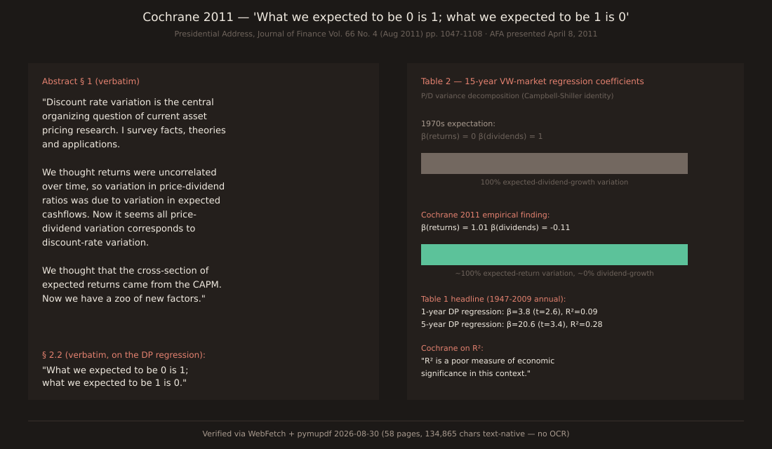
The abstract, verbatim

“Discount rate variation is the central organizing question of current asset pricing research. I survey facts, theories and applications. We thought returns were uncorrelated over time, so variation in price-dividend ratios was due to variation in expected cashflows. Now it seems all price-dividend variation corresponds to discount-rate variation. We thought that the cross-section of expected returns came from the CAPM. Now we have a zoo of new factors. I categorize discount-rate theories based on central ingredients and data sources. Discount- rate variation continues to change finance applications, including portfolio theory, accounting, cost of capital, capital structure, compensation, and macroeconomics.”

Table 1 — DP regression (annual, 1947-2009)

Horizon	β	t(β)	R²
1 year	3.8	(2.6)	0.09
5 years (Hansen-Hodrick correction)	20.6	(3.4)	0.28

Cochrane’s § 2.1 aside (verbatim): “R² is a poor measure of economic significance in this context. The economic question is How much do expected returns vary over time? There will always be lots of unforecastable return movement, so the variance of ex-post returns isn’t a very informative comparison.” The β = 3.8 coefficient is what matters — a 1 pp increase in dividend yield forecasts nearly 4 pp more return next year, the same order of magnitude as the entire equity premium.

Table 2 — 15-year variance decomposition (Campbell-Shiller identity)

Method	β(returns)	β(dividends)	β(dividend yield)
Direct regression, k=15	1.01	-0.11	-0.11
Implied by VAR, k=15	1.05	0.27	0.22
VAR, k=∞	1.35	0.35	0.00

The β(returns) = 1.01 from the direct 15-year regression means 100% of dividend-yield variation translates one-for-one to expected-return variation. The β(dividends) = -0.11is statistically indistinguishable from zero AND has the wrong sign — high P/D ratios don’t forecast higher future dividend growth, they forecast lower future returns.

Cochrane § 2.2 (verbatim): “What we expected to be 0 is 1; what we expected to be 1 is 0.” The 1970s expectation was β(returns) = 0 (efficient markets, no return predictability) and β(dividends) = 1 (all P/D variation reflects future dividend growth). The direct measurement is the exact opposite.

§ 2.3 — Pervasive across markets

“This pattern of predictability is pervasive across markets. For stocks, bonds, credit spreads, foreign exchange, sovereign debt and houses, a yield or valuation ratio translates one-for-one to expected excess returns, and does not forecast the cashflow or price change we may have expected. In each case our view of the facts have changed 100% since the 1970s.”

Cochrane’s Table 3 (§ 2.3) gives side-by-side DP regressions on U.S. houses (1960-2010) and U.S. stocks: houses β = 0.12 (t = 2.52), R² = 0.15; stocks β = 0.13 (t = 2.61), R² = 0.10. “The housing regressions are almost the same as the stock market regressions.” PT #23 AMP 2013 later extended value-momentum across 8 asset classes with the 50/50 combo Sharpe = 1.42 — direct empirical validation of Cochrane’s § 2.3 pervasiveness claim.

The “zoo of new factors” framing

Cochrane § 3 inventories the empirical factor literature that ballooned between 1970 and 2011. CAPM (Sharpe 1964, Lintner 1965) was expected to explain the cross-section of expected returns. Instead, in the subsequent 40 years we accumulated Fama-French 3-factor (1993 — PT #8), Jegadeesh-Titman momentum (1993 — PT #2), Carhart 4-factor (1997 — PT #11), Novy-Marx profitability (2013 — PT #24), plus dozens of others. Cochrane 2011’s “zoo” framing didn’t slow the pace of factor proliferation — 4 years after this address, Fama-French 2015 (PT #22) added two more (profitability RMW and investment CMA), and Harvey-Liu-Zhu (2016) counted 316 published factors by then. The multiple-testing implication is severe: most published Sharpe > 1 factor backtests are almost certainly artifacts of the publication-bias / data-mining ratio, not real risk premia.

Retail-trader takeaways

Three concrete lessons. (1)Yield-based signals ARE predictive of returns across all major markets — stocks, Treasuries, credit, FX, sovereign debt, houses. If a signal shows up in the valuation ratio, it’s about future RETURNS, not future cashflows.

(2)R² is the wrong yardstick for signal usefulness. Cochrane’s 9%R² on 1-year returns is still “huge economic significance” because the coefficient (β = 3.8) is actionable. Same shape as the Vantage News Impact bucket-response tables: today’s Stats #30 showed a tail-to-tail Cohen’s d = +1.51 on US CPI × GBPUSD — VERY LARGE effect size — even though the overall Pearson r is only -0.30 because in_line prints dilute it.

(3)The zoo warning: any single-factor backtest reporting Sharpe > 1 is one of hundreds of similar backtests published in the same window. Cochrane implicitly asks: which of these will replicate out-of-sample? History since 2011 says most won’t — reserve deep skepticism for factor claims that haven’t survived the subsequent 15 years.

Cross-links in the Paper Trail arc

PT #4 Fama 1970 EMH (the 1970s “test market efficiency” framework Cochrane succeeds); PT #2 Jegadeesh-Titman 1993 momentum, PT #8 FF 1993 3-factor, PT #11 Carhart 1997 4-factor, PT #22 FF 2015 5-factor, PT #23 AMP 2013 value-momentum-everywhere, PT #24 Novy-Marx 2013 profitability (all “zoo” factors Cochrane names or directly references); PT #25 FF 2006 (pre-Novy-Marx profitability); PT #26 CGS 2008 (asset growth); PT #27 Sloan 1996 (accruals — the specific PEAD-adjacent anomaly Cochrane cites); PT #28 Piotroski 2000 (F-score value strategy — Piotroski cites Cochrane’s 1999 “New Facts in Finance” the paper immediately preceding this one). Same intellectual lineage all the way through.

Verification note

Primary source obtained via WebFetch of igier.unibocconi.eu/sites/default/files/media/attach/AFA_pres_speech.pdf, rendered to text via pymupdf 1.28 on 2026-08-30. Full 58-page text-native extract (134,865 characters, no OCR required). Abstract, Table 1, Table 2, Table 3, § 2.2 aphorism, § 2.3 pervasive- markets list, and § 3 zoo-of-factors framing all verified verbatim against the extracted text. DOI matches Wiley Online Library (10.1111/j.1540-6261.2011.01671.x → Journal of Finance Vol. 66 No. 4 pp. 1047-1108). 22nd Paper Trail out of 30 with full primary- source access. Chart via a scratch script reusing scripts/insights-charts/svg.ts and theme.ts primitives with sharp rasterization (not committed under scripts/).

Keep reading