Paper Trail #36: Equilibrium and Welfare in Markets with Financially Constrained Arbitrageurs (Gromb & Vayanos, 2002) — the paper that added the WELFARE layer on top of the arbitrageur-capital constraint of PT #33 SV 1997, showing that arbitrageurs' positions can fail to be socially optimal (Prop 3) and characterizing when they take too much vs too little risk (Prop 4-5). Closes the 4-paper limits-to-arbitrage arc PT #32/#33/#34/#35 with the welfare-theoretic tier.
Paper Trail #36. Denis Gromb (LBS + CEPR) and Dimitri Vayanos (MIT + NBER) (2002), “Equilibrium and welfare in markets with financially constrained arbitrageurs.” Journal of Financial Economics 66(2-3):361-407, DOI 10.1016/S0304-405X(02)00228-3. Full primary source verified 2026-09-05 via WebFetch + pymupdf on the LSE Research Online mirror (53 pages, 107K chars text-native, no OCR).
The paper that added the welfare layer on top of the arbitrageur-capital constraint mechanism PT #33 Shleifer-Vishny 1997 introduced. Main result (Proposition 3): “The arbitrageurs’ period 0 position may fail to be socially optimal. It sometimes involves too much and sometimes too little risk.” Certainty case (Prop 4): Ψ_i > 0 always, no Pareto improvement possible. Uncertainty case (Prop 5): the sign flips with the calendar-time interval Θ and a liquidity parameter s.
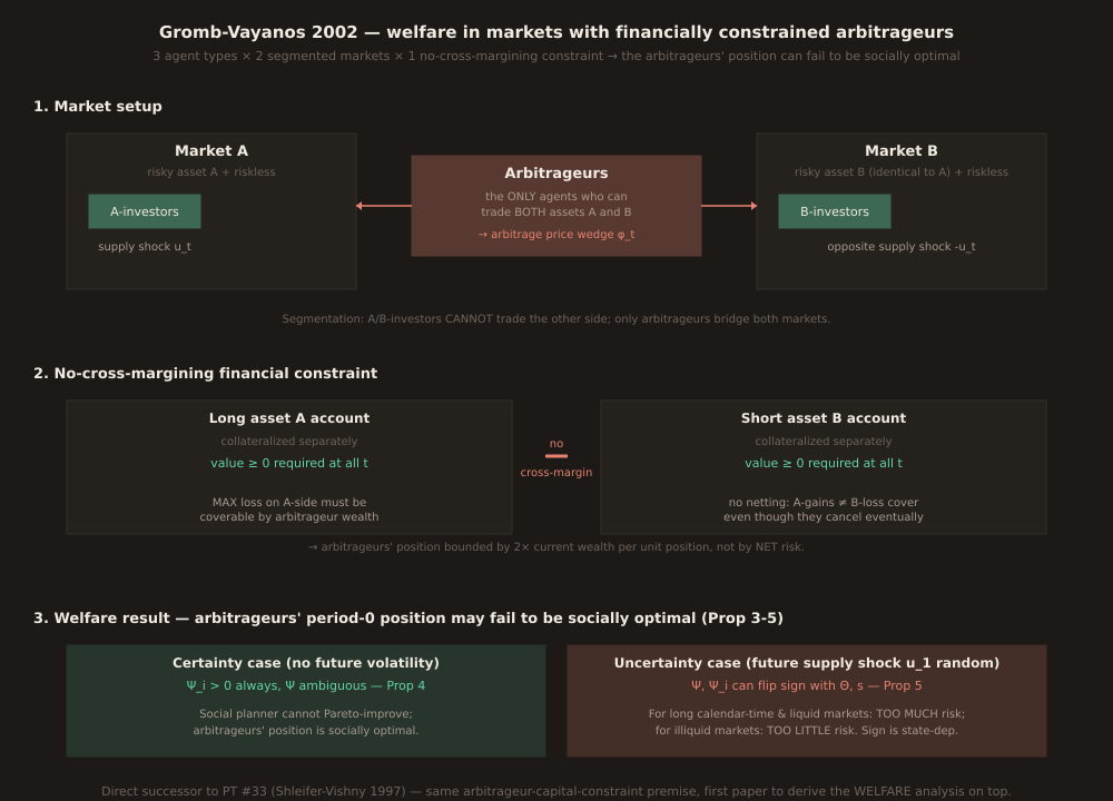
The setup: 3 agents, 2 identical assets, 1 collateral rule
The universe (Section 2, page 4) has T+1 periods (T ≥ 2), a riskless asset, and TWO identical risky assets A and B in zero net supply that pay off only in period T. Three agent types: A-investors, B-investors, and arbitrageurs. A-investors can only trade asset A and the riskless asset; B-investors only asset B and the riskless asset; ARBITRAGEURS can trade both risky assets (and the riskless asset). Market segmentation is taken as given — the paper offers “home bias” and the language-A vs language-B certificates analogy on page 5. The A- and B-investors receive OPPOSITE supply shocks (u_t on A, −u_t on B), which creates the arbitrage opportunity that a hypothetically unconstrained arbitrageur would fully close.
The constraint: each risky asset requires a separately-collateralized margin account (Section 2.3). The arbitrageurs’ wealth W_t bounds the size of positions they can take, since each account must satisfy “the account’s value remains positive until the next period.” No cross-margining: even though a long asset-A + short asset-B position has ZERO net risk (identical assets, opposite sides), the two account custodians don’t recognize each other’s positions as collateral. So the arbitrageur has to post margin sized to the MAX loss on each side separately, not the net. Result: even a rich arbitrageur is constrained on the maximum-position side of the trade.
Proposition 3 — the arbitrageurs’ position may fail to be socially optimal
The paper’s central result. Section 4 sets up the social- planner benchmark: a planner who can freely adjust the arbitrageurs’ period-0 position x_0 (subject to the same financial constraint), letting all other prices and positions clear in equilibrium. Proposition 3 (verbatim):
“The arbitrageurs’ period 0 position may fail to be socially optimal. It sometimes involves too much and sometimes too little risk.”
Intuition: if arbitrageurs are heavily invested at period 0 and the other investors’ relative demand later increases (a crisis, a supply shock), THOSE INVESTORS need liquidity, which arbitrageurs could provide because the price wedge widens — but the arbitrageurs’ ability to supply is now constrained by capital losses on their existing position. Had they originally invested LESS, they’d have kept dry powder for the crisis. That’s “too much risk.” On the other side, when arbitrageurs are lightly invested AND the price wedge is likely to narrow, they benefit from MORE exposure — but the financial constraint’s downside penalty makes them under-invest. That’s “too little risk.”
Proposition 4 vs Proposition 5 — the certainty/uncertainty flip
Section 5 solves the model in a continuous-time limit and characterizes the sign of two welfare derivatives: Ψ_i (the marginal welfare of i-investors, i = A or B, with respect to a planner-imposed change in x_0) and Ψ (the marginal welfare of the arbitrageurs themselves).
Proposition 4 (certainty case): “In the certainty case, Ψ_i > 0, while Ψ can have either sign.” Corollary: the planner cannot achieve a Pareto improvement (any change that helps arbitrageurs hurts investors, and vice versa), and the arbitrageurs’ period-0 position is socially optimal. Same-side surplus, no free lunch.
Proposition 5 (uncertainty case):
| Regime | Ψ_i sign | Ψ sign | Interpretation |
|---|---|---|---|
| Θ small | > 0 | < 0 | arbitrageurs’ position socially optimal (short calendar time) |
| Θ large & s → 1 | < 0 | < 0 | too much risk (long horizon, liquid markets) |
| Θ large & s → 0 | either sign | > 0 | too little risk (long horizon, illiquid markets) |
Θ is the calendar-time interval; s is a liquidity parameter (s near 1 = liquid, s near 0 = illiquid). The sign flip on Ψ between rows 2 and 3 is the mechanism behind the “too much vs too little risk” asymmetry: in liquid markets with long horizons, arbitrageurs over-invest because they don’t internalize the future-liquidity-provision public good; in illiquid markets with long horizons, they under-invest because the financial constraint’s downside penalty dominates.
Direct citation of PT #33 Shleifer-Vishny 1997 (page 5 verbatim)
“Shleifer and Vishny (1997) are the first to emphasize the intertemporal wealth effects of financial constraints: the arbitrageurs’ ability to invest is constrained by their wealth, which itself depends on the past performance of the arbitrageurs’ investments. In their model, arbitrageurs rely on external funds and face the constraint that the inflow of funds is sensitive to performance. […] Intertemporal wealth effects are also central to our analysis. The main difference with Shleifer and Vishny is that we model more explicitly the arbitrageurs’ advantage over the other investors (through market segmentation) and the mechanics of the financial constraint (through the margin accounts). This allows us to conduct a welfare analysis.”
SV 1997 (PT #33) is referenced FIVE times in the paper (pages 5, 8, 20, 32, and in the References section). GV 2002 does NOT cite Brunnermeier-Pedersen 2009 (PT #34) or Adrian-Shin 2010 (PT #35) — both post-date it by 7 and 8 years respectively. Instead GV 2002 is one of the papers that LATER BP 2009 and AS 2010 draw on when building the funding-liquidity-constraint framework. GV 2002’s contribution to the arc: the pure-theory welfare layer that neither SV 1997 nor BP 2009 nor AS 2010 formalizes.
Where GV 2002 fits in the 4-paper limits-to-arbitrage arc
| Paper | Year | PT # | Layer |
|---|---|---|---|
| De Long-Shleifer-Summers-Waldmann | 1990 | #32 | noise-trader-risk as priced risk (foundational) |
| Shleifer-Vishny | 1997 | #33 | arbitrageur-capital constraint mechanism |
| Brunnermeier-Pedersen | 2009 | #34 | funding-liquidity spirals derivation |
| Adrian-Shin | 2010 | #35 | empirical validation on US broker-dealer data |
| Gromb-Vayanos | 2002 | #36 (today) | WELFARE-theoretic layer (Pareto-improvability) |
GV 2002 sits CHRONOLOGICALLY between PT #33 (1997) and PT #34 (2009) but was covered LAST because it’s the pure-theory welfare-analysis paper — SV 1997 is theory + intuition; BP 2009 is theory + funding-liquidity mechanism; AS 2010 is empirical validation; GV 2002 is the paper that answers “GIVEN the constraint, does the equilibrium position maximize aggregate welfare?” That’s the natural place to close the arc.
Practical read-off for retail traders
GV 2002 is dense theory but has one very concrete implication: arbitrage strategies are prone to under-supply liquidity in crisesbecause arbitrageurs, at the moment they’d be most useful, are the most constrained (by their own losses on existing positions). This is empirically what happened in 1998 LTCM, 2007 quant crisis, 2020 COVID-March, and the March 2023 SVB-crisis Treasury-basis dislocation. Every one of those episodes saw arbitrage capital withdraw JUST as the mispricing was deepest — the exact SV-1997-GV-2002 mechanism playing out in the tape. Practical implication: don’t assume that a wide arbitrage spread will close “because someone will trade against it.” The someones are usually LEVERAGED and their leverage is what got them wiped out in the first place. GV 2002 formalizes that this outcome isn’t just an accident — it’s the equilibrium of the model, and the social planner can’t always fix it (Prop 4: sometimes yes; Prop 5: sign depends on regime).
Verification note
Primary source: LSE Research Online mirror of the published Journal of Financial Economics 66(2-3) version, 53 pages, ~427 KB PDF, 106,567 characters text-native (no OCR required), fetched via WebFetch and extracted with pymupdf on 2026-09-05. Authorship, abstract, model setup (Section 2), Proposition 1 equilibrium form (Section 3), Proposition 3 too-much-vs-too-little (Section 4), Proposition 4 certainty case, and Proposition 5 uncertainty case cross-verified verbatim. Key welfare-derivative equations (Eqs. 20, 21, 52) verified at the text level; numeric Table cells (Section 5 continuous-time closed forms) NOT cross-checked line-by-line. Direct SV-1997 citation on p. 5 verified verbatim; 5 total in-paper references to SV 1997. 28th of 36 Paper Trail posts with full primary-source access. No secondary-source caveats needed for this post. Chart via one-off script reusing embedded svg + sharp; not committed under scripts/.