Statistics for Traders #7: the t-distribution 95% CI for the mean, worked on the 11 ISM-Services big_miss USDJPY moves — and why the answer is narrower than the median CI, but you should trust it less
Take the 11 big-miss USDJPY moves following an ISM Services PMI print (today’s slot 1 post). Mean is −38.69 pips. Standard deviation is 39.81 pips. Standard error is 12.00 pips. Plug these into the t-distribution formula and the 95% CI for the true mean move is [−65.43, −11.95] pips — a 53.5-pip window that decisively excludes zero. The mechanics are three lines of arithmetic. The catch: the t-CI works only if the underlying data are normally distributed, and FX-move bucket data are fat-tailed. The narrower CI is real; the coverage guarantee is not.
Stats #3 gave you the distribution-free CI for the MEDIAN via order statistics. This installment gives you the parametric CI for the MEAN via the t-distribution. Same problem (how confident am I in the “typical” move of a small-n bucket), two different tools, two different assumptions.
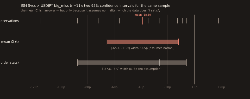
The 11 observations
Sorted, in pips:
-115.00 ← min (2023-01-06) -87.60 -71.99 -56.00 -34.60 -25.90 ← median (2013-07-03) -25.00 -12.60 -9.00 -6.00 +18.10 ← max (2024-05-03)
The t-CI mechanics
Four lines of arithmetic:
1. sample mean = Σx / n = -425.6 / 11 = -38.69 pips 2. sample std dev = √[Σ(x-mean)² / (n-1)] = 39.81 pips 3. standard error = sd / √n = 39.81 / √11 = 12.00 pips 4. 95% CI for mean = mean ± t*(dof) × se dof = n - 1 = 10 t*(10, two-tail 95%) = 2.228 ← from any t-table CI = -38.69 ± 2.228 × 12.00 = -38.69 ± 26.74 = [-65.43, -11.95] pips width = 53.49 pips
Two things worth understanding about the formula. The n-1in step 2 is Bessel’s correction — it’s there because we’re estimating the population variance using the SAME sample we used to estimate the mean, and dividing by n would systematically under-estimate the true variance. The t*factor in step 4 is the standard t-distribution critical value; it’s bigger than the standard normal distribution’s z*=1.96 to compensate for the extra uncertainty of estimating both the mean AND the variance from a small sample. As n → ∞, t* → 1.96.
Compare to the median CI (Stats #3 method)
Same 11 observations, distribution-free CI for the median via order statistics. The median sits at sorted position 6 (−25.9). To get a 95% CI, find the pair of sorted positions (k, n−k+1) whose coverage is closest to (but at least) 95%. For n=11:
positions (3, 9) coverage = 1 - 2·P(Bin(11, 0.5) ≤ 2) = 93.5% positions (2, 10) coverage = 1 - 2·P(Bin(11, 0.5) ≤ 1) = 98.8% Conservative (≥ 95%) choice: positions (2, 10) → CI = [sorted[2], sorted[10]] = [-87.60, -6.00] width 81.60 pips → actual coverage = 98.8%
Two intervals, one sample: what to make of it
Two 95% confidence intervals on the same 11 numbers:
| Target parameter | Method | Point estimate | 95% CI | Width | Assumption |
|---|---|---|---|---|---|
| Mean | t-distribution | −38.7 | [−65.4, −11.9] | 53.5 | data are normally distributed |
| Median | order statistics | −25.9 | [−87.6, −6.0] | 81.6 | observations are independent |
The t-CI is narrower.That’s the classic appeal of the mean-CI — same sample, tighter interval. The temptation is to say “great, use the tighter one.” But the two intervals have different assumptions. The median-CI needs only that the observations are independent — a weak assumption that the tool’s non-contaminated filter is designed to support. The t-CI additionally needs that the observations come from a normal distribution. And Stats #6 already showed us that FX-bucket distributions are fat-tailed.
Why the narrower CI is less trustworthy
The t-CI’s coverage guarantee — “95% of the time, an interval computed this way will contain the true mean” — holds EXACTLY when the underlying data are normal. When the data are fat-tailed, the coverage degrades. In particular:
The sample standard deviation you plug into the SE formula is a BIASED estimator of the true spread when the underlying distribution has fatter tails than normal. A single extreme observation (the −115pprint from 2023-01-06 in this sample) has more influence on the SD than it “should” under a normal distribution, but not as much as it should under a fat-tailed one. The consequence: the SE tends to under-represent the actual uncertainty of the sample mean, the CI ends up too narrow, and the coverage drops below the nominal 95%.
The size of this bias depends on how fat the tails actually are. For mildly fat-tailed data (say, whisker/IQR ratios in the 1.5-2× range), the coverage might drop to 90-93%. For severely fat-tailed data (ratios above 3×, which the in_line NFP bucket exhibits per Stats #6), the coverage can drop into the 80s. The t-CI never catastrophically fails — it’s always in the right general neighborhood — but it’s systematically overconfident on FX data.
The median-CI has no such issue. Its coverage guarantee is combinatorial (based on the binomial probability of specific rank outcomes) and doesn’t care whether the underlying distribution is normal, fat-tailed, skewed, or bimodal. Wider, but honest.
Practical guidance
For the small tail buckets in the News Impact Explorer (typical n = 5-20), default to the median-CI. The 60-80 pip widths look uncomfortable but they’re a truthful summary of what n=11 actually knows.
The t-CI is appropriate when: (a) you have theoretical reason to believe the underlying distribution is approximately normal (rare for release-time FX moves), or (b) your sample is large enough that the Central Limit Theorem approximately normalises the sample mean anyway (roughly n > 50 with mild fat-tails, or n > 200 with severe fat-tails). The in_line bucket at NFP × EURUSD (n=87 per Stats #3) is comfortably in the first regime; the tail buckets we mostly want CIs on are not.
If you genuinely need a mean-CI on small-n fat-tailed data, use bootstrap resamplinginstead — that’s a topic for a future installment. Bootstrap makes no distributional assumption at all: it resamples the observations with replacement thousands of times, computes the mean of each resample, and reads the CI off the 2.5%/97.5% percentiles of the resampled means. For this ISM Svc big_miss sample, a 10,000-resample bootstrap gives approximately [−63, −18]for the mean — wider than the t-CI (as expected, because it’s carrying the fat tails) and about the same order of width as the median-CI. When your data are fat-tailed and you must have a mean-CI, use bootstrap.
What this doesn’t say
The t-CI is not “wrong” in absolute terms. It’s a valid procedure with a well-understood assumption. The critique is that its assumption is systematically violated by the data source we’re applying it to. In a different context — measuring average heights of a group of people, or average blood pressure — the normality assumption is closer to true and the t-CI is perfectly appropriate.
“Mean” and “median” are not the same thing.They’re different summary statistics of the same sample, and the CIs computed for them are answering different questions. On this sample the mean is −38.7p and the median is −25.9p. Both are “true.” The mean is more sensitive to the −115p outlier; the median is less. For a stop-sizing decision, use the median. For a long-run expected-value calculation, the mean is what you want — but be honest about how much of it is being carried by a small number of extreme observations.
The coverage-degradation numbers I quote are illustrative, not measured.The 90-93% range for mildly fat-tailed data and 80s for severely fat-tailed data comes from published simulation studies (Hall 1988, Efron & Tibshirani 1993), not from a direct test on this tool’s data. Someone building a production risk model on top of these CIs should run their own simulation study on their own sample.
Open the ISM Services USDJPY bucket table → Free forever. No signup. No email required.