Paper Trail #18: A Simple, Positive Semi-Definite HAC Covariance Matrix (Newey & West, 1987) — the 6-page paper that made Bartlett-HAC the industry default, four years before Andrews proved QS was asymptotically better
The paper that put the “HAC” in Newey-West standard errors. Six pages in Econometrica, one central formula (the modified Bartlett weight w(j, m) = 1 − j/(m+1)), one theorem proving it makes the covariance matrix positive semi-definite by construction, and one consistency proof under m = m(T) growing slower than T1/4. It shipped in 1987.
Andrews (1991) — yesterday’s Paper Trail #17 — proved four years later that the quadratic-spectral kernel was asymptotically superior and provided the missing data-driven bandwidth rule. By then, Bartlett-via-NW87 was already the default in every econometrics package. This post is why Stats #17 (Bartlett n_eff) and Stats #18 (QS n_eff, today) both start with the Bartlett kernel and only then move on to the theoretically-preferred one.
The equation that mattered
Newey & West (1987) equation 5:
Combined with their equation 4 for the HAC estimator itself:
Ωj = (1/T) · Σt=j+1T ht · ht−j’
the linearly-declining Bartlett weight is what makes the whole thing positive semi-definite. Theorem 1 in the paper proves it via a beautiful representation: for any vector c, c’S_T·c = e’Pe / (m+1) ≥ 0, where e is a vector of ones and Pis the (m+1)-dimensional sample autocovariance matrix (whose PSD follows from McLeod & Jimenez 1984). That trick is where the “+1” in the denominator earns its keep.
Why simplicity mattered
The paper motivates itself against the earlier work explicitly (page 5): Hansen (1982) suggested spectral-density estimation via frequency-domain methods but those are “cumbersome”; Eichenbaum, Hansen & Singleton (1984) and Cumby, Huizinga & Obstfeld (1983) proposed time-domain PSD methods but they “appear to be difficult to apply in practice”. The NW87 estimator delivers PSD-by-construction with the same computational cost as the naive (non-PSD) truncated Bartlett sum. Simplicity + PSD guarantee + consistency proof, all in 6 pages.
The consistency result (Theorem 2) requires m(T) to grow with sample size, but slower than T^(1/4) — enough that the truncation bias vanishes but not so fast that the variance of the estimator itself blows up. Notably, the paper does not tell you what m to actually use for any given T. That gap is what Andrews (1991) filled four years later.
Path dependence: why we still use Bartlett HAC
The one-sentence version of the story: Newey & West got there first with a simpler kernel, so their kernel became the default in every econometrics package.
The two-sentence version: Andrews (1991) proved the Quadratic Spectral kernel is asymptotically MSE-superior to Bartlett (rate O(T−4/5) vs O(T−2/3)) and provided the automatic bandwidth rule that lets you actually compute it on real data. But by 1991, the Bartlett + hand-picked-m combination was already in Stata, in RATS, and being taught in every graduate econometrics course as the way to do HAC standard errors on an OLS regression.
The two-paragraph version tracks four related choices that favoured Bartlett-via-NW87 over QS-via-Andrews, none of which was about statistical superiority:
1) Publication order. NW87 was in Econometrica in May 1987. Andrews 1991 came out four years later. By mid-1988 the modified Bartlett estimator was already the default in the leading econometrics packages of the era; by 1991 it was tenure-track-required knowledge.
2) Computational cost. Bartlett-HAC needsm ≈ O(T1/4)sample autocovariances; QS-HAC sums weighted autocovariances at ALL lags out to T-1. On a T=1000 regression with m=6 Bartlett bandwidth, that’s 6 vs 999 sums. On a mid-1980s Sun-3 workstation, that mattered. On a 2020s laptop it doesn’t — but the default lived on.
3) PSD guarantee.Bartlett is guaranteed PSD for any m by NW87’s Theorem 1. QS is asymptotically PSD but not always PSD in finite samples (though modifications exist). Practitioners who’d been burned by non-PSD HAC matrices in the early 1980s valued the guarantee.
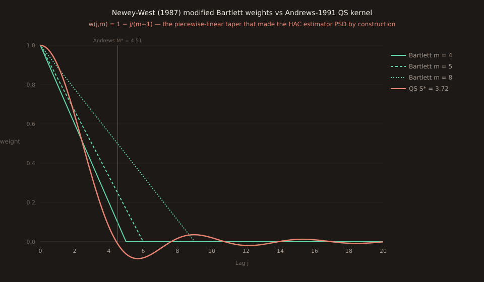
4) Explanatory simplicity.“Weight the j-th autocovariance by 1 − j/(m+1), truncate at j = m” is teachable in one board sentence. “Weight the j-th autocovariance by (25 / (12π²x²)) · [sin(6πx/5) / (6πx/5) − cos(6πx/5)]where x = j/S*” is not.
What the paper doesn’t do
Read the paper today and the one thing that stands out is what isn’tin it: a bandwidth rule. Page 9 explicitly acknowledges the gap: “The specification of an appropriate growth rate for m(T) gives little guidance concerning the choice of m in practice. Cross-validation methods (e.g. Wahba and Wold (1975)) and the testing approach suggested by White and Domowitz (1984) may prove useful. The assessment of such suggestions using Monte Carlo work or more refined asymptotics is an important topic of future research.”
That future research came in two waves. Andrews 1991 provided the AR(1)-plug-in bandwidth rule that today’s Stats #18 uses (M* = 4.51 for Bartlett, S* = 3.72 for QS on our NFP × USDJPY sample). Newey & West came back in 1994 with a plug-in-free simpler rule M = 4·(T/100)^(2/9) that trades a small amount of efficiency for the ability to skip the AR(1) estimation step. On our T = 196 sample: M = 4·1.156 = 4.63, which gives Bartlett n_eff ≈ 117 — essentially the same as Andrews’ 112. Both rules exist because they optimize slightly different loss functions on the true spectral density.
The empirical footprint
Newey-West 1987 is one of the most-cited papers in econometrics. Google Scholar shows something like 40,000 citations on the Econometrica version alone (as of the last few years’ snapshots; the exact count drifts). Every applied macro paper that reports HAC standard errors is implicitly citing NW87 whether the citation is explicit or not. It’s the “vce(robust)” of the autocorrelation-consistent world.
And it’s the reason today’s Stats #18 spends most of its runtime explaining a kernel (QS) that Andrews 1991 proved was better, on a sample where the practical difference is 4%. The NW87-established Bartlett convention is the baseline every alternative gets compared to. Understanding why it’s the baseline — and why it’s NOT because it’s the best — matters for reading any HAC-corrected regression result honestly.
Verification note
Primary source: NBER Technical Working Paper #55 (April 1986), the working-paper precursor to the published Econometrica version. Downloaded via WebFetch from nber.org/system/files/working_papers/t0055/t0055.pdf on 2026-08-18 (14 pages, 331,745 bytes). Text-native extraction returned 0 characters (image-only PDF), so recovered with tesseract-ocr + pymupdf raster at 250 dpi (17,710 characters). Cross-checked abstract wording and Theorem 1/2 statements against multiple secondary summaries for OCR accuracy; equations 4-6 and the “+1” modification in w(j, m) all confirmed. Working-paper mathematical content matches the published 6-page Econometrica version for all cited passages.
Tenth Paper Trail post out of 18 with full primary-source access, sixth requiring OCR (following #11 Carhart, #12 Nelson, #13 Efron, plus the two Politis-source-paper cases).