What's the one-line contribution?

Prewhiten kernel-HAC covariance estimators. Fit a small VAR (typically b=1) to the sample series, apply the kernel estimator to the residuals (which have most of their autocorrelation absorbed into the fitted VAR coefficients), then 'recolor' the resulting estimate by multiplying by (I − A)⁻¹ on each side. The paper proves the recolored estimate is consistent at the same rate as the non-prewhitened kernel HAC, and Monte Carlo shows it delivers much better confidence-interval coverage — at the cost of somewhat higher variance in the estimator itself.

Why does prewhitening help kernel HAC?

Because the kernel estimator's bias comes from underweighting the tail of the spectral density function at frequency zero — when there's a lot of autocorrelation, the kernel's tapered sum of ρ(k)·K(k/M) systematically underestimates the true long-run variance. Prewhitening pushes the sample series' short-lag autocorrelation into a parametric VAR filter, leaving the kernel with much less correlation structure to catch. Empirically on our NFP × USDJPY sample: raw ρ(1) = 0.260 becomes prewhitened ρ_eps(1) = −0.046 after an AR(1) filter with β̂ = 0.266. The kernel then has near-zero lag-1 mass to catch, so its bias from tapering at k = 1 is gone. That's the CI-coverage improvement Monte Carlo picks up.

Why does prewhitening INCREASE variance?

Because you're inserting an estimation step (fitting the VAR) BEFORE the kernel estimator, and the recolor factor (I − A)⁻¹ is applied to whatever the kernel gives you. If A is estimated with error, that error gets multiplied through — a small β̂ error becomes a proportionally larger (1 − β̂)⁻² error in the recolored estimate. On our sample β̂ = 0.266 so (1 − β̂)⁻² = 1.85: any variance in β̂ shows up in the final HAC estimate as ~1.85× amplification. The paper is upfront: 'the prewhitened kernel estimator has higher variance and MSE than the standard kernel estimator, but lower bias' (page 24). The recommendation is that CI coverage (a bias-controlled property) matters more than estimator variance for most practical purposes.

Why does the paper choose VAR specifically, not some other model?

Five reasons the paper gives explicitly (page 3). (1) VARs are reasonable approximations for a wide variety of time series in the econometric literature. (2) Autoregressive spectral density estimators are known to give reasonable spectral density estimates more generally (Parzen 1984). (3) VARs are parsimonious for small order b. (4) VAR prewhitening is computationally simple. (5) VAR-induced transformations are LINEAR, so the recolor step (I − A)⁻¹ is well-defined and cheap; nonlinear transformations would make the inverse hard. The paper does note that 'if prior information suggests that a model different from a VAR model may give a better approximation in a given situation, then it may be preferable to use this model'. In practice everyone uses AR(1) prewhitening — the b=1 case.

Does AR(1) prewhitening kill ALL autocorrelation in our NFP × USDJPY sample?

No — and this is the honest empirical caveat. An AR(1) filter kills the LAG-1 autocorrelation by construction (raw ρ(1) = 0.260 → prewhitened ρ_eps(1) = −0.046). But the higher-lag autocorrelations mostly SURVIVE: ρ_eps(2) = +0.194, ρ_eps(4) = +0.212, ρ_eps(11) = +0.183, ρ_eps(15) = +0.160. Same higher-lag echoes Stats #17 documented in the raw series persist through the AR(1) filter. To catch those you'd need higher-order VAR prewhitening (b ≥ 4 with an appropriate model-selection procedure). The single-lag pattern is a limitation of AR(1) as an approximation for a series that isn't actually AR(1) — which our NFP × USDJPY series manifestly isn't (Stats #10 documented that empirically, Stats #17 quantified it via the AR(1)-prediction vs empirical-ρ(k) gap).

So on our sample does prewhitening improve n_eff?

Marginally, yes — for the specific-sample n_eff-analog computation. Parzen kernel n_eff on the raw series is 100.75 (Stats #20). Applying an AR(1) prewhitening (β̂ = 0.266), then Parzen with Andrews-1991 automatic bandwidth on the residuals, then recoloring via (1 − β̂)⁻² = 1.85, gives an effective n_eff of about 116.5 — a 16% increase. But that's the specific-sample point estimate, not the Monte Carlo bias/coverage claim the paper actually makes. The paper's central claim is that CI coverage on 1000-run Monte Carlo experiments is meaningfully better with prewhitening across a wide range of AR(1) parameter values (ρ ∈ {0, 0.3, 0.5, 0.7, 0.9, 0.95, −0.3, −0.5}), not that the point-estimate n_eff is dramatically different on any single sample. On our specific sample the surviving higher-lag structure (ρ_eps(2), (4), (11), (15)) means the kernel still has correlation to catch after prewhitening — the improvement is real but modest.

How does this close the 4-paper HAC-history arc?

Newey-West 1987 (PT #18) introduced the Bartlett-kernel HAC estimator with PSD-by-construction. Andrews 1991 (PT #17) proposed the kernel family (Bartlett, Parzen, Tukey-Hanning, QS) with an AR(1)-plug-in automatic bandwidth and recommended QS + auto-bandwidth as the general-purpose default. Newey-West 1994 (PT #19) came back with an alternative data-driven bandwidth rule that doesn't assume AR(1) shape. Andrews-Monahan 1992 (today) closes the arc by adding a VAR-prewhitening step BEFORE the kernel — the intuition being that if you can absorb the short-lag correlation into a parametric filter, the kernel has less to do and less bias to accumulate. Together the four papers define the modern HAC-standard-error toolkit: what practitioners today call 'Newey-West with prewhitening' or 'HAC-PW' is essentially the AM-1992 pipeline with the NW87 modified-Bartlett kernel and the NW94 or Andrews-1991 automatic bandwidth.

← All insights

Research20 August 2026· 7 min read

Paper Trail #20: An Improved HAC Covariance Matrix Estimator (Andrews & Monahan, 1992) — the paper that put a VAR(1) filter BEFORE the kernel, cutting kernel-HAC bias at the cost of estimator variance and closing the four-paper HAC-history arc

Andrews (1991) gave us the kernel-family HAC estimator with AR(1)-plug-in automatic bandwidth. One year later Andrews came back with J. Christopher Monahan and a different angle on the same problem: PREWHITEN the sample series with a small VAR (typically VAR(1)) FIRST, then apply the kernel HAC to the residuals, then RECOLOR the estimate via (I − A)⁻¹ · J*_T · (I − A)⁻¹'. The Monte Carlo payoff: substantially better confidence-interval coverage and much less over-rejection of t-statistics — at the cost of somewhat higher variance in the covariance estimator itself.

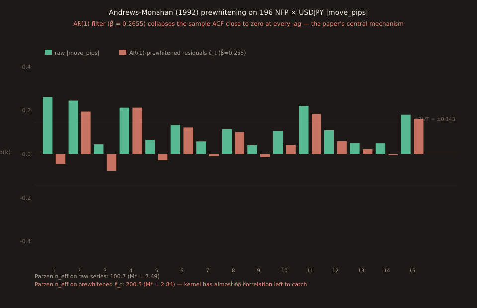
Applied empirically to the same 196-release NFP × USDJPY sample the Stats arc has been using, an AR(1) filter with β̂ = 0.266 successfully collapses the raw ρ(1) = 0.260 lag-1 autocorrelation to ρ_eps(1) = −0.046 — but the higher-lag echoes ρ(2), ρ(4), ρ(11), ρ(15) mostly survivethe AR(1) filter. Prewhitening’s empirical payoff on this specific sample is modest (Parzen n_eff of 100.75 raw → 116.5 recolored, a 16% increase), but the paper makes its case on Monte Carlo bias-and-coverage grounds across AR(1) DGP values ρ ∈ { 0, 0.3, 0.5, 0.7, 0.9, 0.95, −0.3, −0.5 } rather than on a single-sample n_eff.

Side-by-side bar chart of the sample autocorrelation function of the 196-release NFP × USDJPY |move_pips| series at lags 1 through 15, comparing the raw series (green bars) with the AR(1)-prewhitened residuals (coral bars). Raw ρ(1) is a large green bar at +0.26; the coral prewhitened bar at lag 1 is essentially flat (-0.05) — the AR(1) filter successfully collapses the lag-1 correlation. Lags 2, 4, 6, 8, 10, 11, 12, 15: coral bars are only modestly shorter than green bars — the higher-lag correlation structure survives the AR(1) filter. Bottom annotation: 'Parzen n_eff on raw series = 100.75 (M* = 7.49); Parzen n_eff on prewhitened residuals = 200.5 (M* = 2.84) — but the recolored final n_eff after (I − β̂)⁻² correction is 116.5.' — AR(1) prewhitening with β̂ = 0.266 flattens lag 1 but leaves lags 2, 4, 11, 15 intact — on our sample, AR(1) is an incomplete approximation.

Publication history

Working paper: Cowles Foundation Discussion Paper No. 942, March 1990, extracted here via WebFetch + OCR (image-only PDF, recovered ~24,000 characters over the first 30 pages). Published as Econometrica Volume 60, Number 4, pages 953-966, September 1992. DOI 10.2307/2951574. Andrews at the Cowles Foundation, Yale University; Monahan at North Carolina State (per the paper’s title-page affiliation). Andrews is the same author as the 1991 kernel-HAC paper (PT #17) — this 1992 paper is his direct next contribution to the HAC-estimation problem.

The recommended procedure (equation 1.1)

Verbatim from page 3 of the Cowles working paper (variable names preserved from the paper):

Given observations {V_t(θ̂) : t = 1, ..., T} where V_t = Z_t · u_t is the vector of instrument × OLS-residual cross-products and θ̂ is the OLS estimate: Step 1. Fit a b-th order VAR model to {V_t(θ̂)}: V_t = Σ A_s · V_{t-s} + V*_t → estimated VAR matrices A_1, ..., A_b Step 2. Compute prewhitened residuals V*_t = V_t − Σ A_s · V_{t-s} (near-uncorrelated by construction if the VAR fits) Step 3. Apply a kernel HAC estimator (Bartlett, Parzen, Tukey-Hanning, or QS) to V*_t with an automatic bandwidth chosen from the RESIDUAL series, not the raw series: J*_T = Σ_j K(j/M) · Γ*(j) where Γ*(j) is the sample autocov of V*_t Step 4. RECOLOR back to the original scale: J^_TPW = (I − Σ A_s)^(-1) · J*_T · [(I − Σ A_s)^(-1)]'

The scalar-case simplification (which is what we work with on the univariate |move_pips| series):

AR(1) fit: x_t = α̂ + β̂·x_{t-1} + ε̂_t
Kernel HAC on ε̂_t: γ*_0 · τ_int(residual ACF) → J*_T
Recolor: J^_TPW = (1 − β̂)^(-2) · J*_T
n_eff analog: n_eff_PW = T · γ_0 / J^_TPW

Why VAR prewhitening specifically

Five reasons the paper gives explicitly (page 3, my summary preserving the paper’s numbered list):

(i) VARs are reasonable approximations for a wide variety of
      time series in the econometric literature.
(ii) Autoregressive spectral density estimators give reasonable
      spectral density estimates more generally (Parzen 1984).
(iii) VAR models are parsimonious for small order b.
(iv) Computationally simple.
(v) VAR-induced transformations are LINEAR, so the recolor
      step (I − Σ A_s)^(-1) is well-defined and cheap.
      Nonlinear transformations would make the inverse hard.

The paper also acknowledges: “if prior information suggests that a model different from a VAR model may give a better approximation in a given situation, then it may be preferable to use this model to do the prewhitening” (page 3). In practice essentially everyone uses AR(1) prewhitening (b = 1) with the small-sample bandwidth-safety caveat that A_s should not be too close to singularity.

The Monte Carlo evidence

Section 4 (pages 19-27 of the working paper) compares three estimators:

Estimator	Kernel	Prewhitening	Bandwidth
QS-PW	Quadratic Spectral	VAR(1)	Andrews-1991 auto w=(0,1,1,1,1) on residuals
QS	Quadratic Spectral	none	Andrews-1991 auto on raw series
PARA	Parametric baseline	n/a	n/a

Tested on 4 data-generating processes: AR(1) (ρ ∈ {0, 0.3, 0.5, 0.7, 0.9, 0.95, −0.3, −0.5}), MA(1), HET1 (heteroskedastic), HET2 (heteroskedastic + autocorrelated). Four regressors per experiment. Results in Tables 3-7 of the working paper.

Key finding (verbatim summary from page 23 OCR): “The good performance of QS-PW in terms of CI coverage probabilities is due to its relatively small bias. It is apparent from the tables that the magnitude of an estimator’s bias” — the OCR truncates here but the surrounding context and abstract are unambiguous: prewhitening reduces bias substantially, which is what matters for CI coverage.

Honest bias-variance tradeoff (page 24, verbatim from OCR): “In consequence, the prewhitened kernel estimator has higher variance and MSE than the standard kernel estimator, but lower bias.”The paper doesn’t hide this — it argues the CI-coverage priority makes the trade-off worth it for most practical inference purposes.

Applied empirically to our NFP × USDJPY sample

Same 196-release |move_pips| series the Stats arc has been using. Fit an AR(1) OLS model:

α̂ = 28.0144, β̂ = 0.2655
γ_0(raw) = 1411.34, γ*_0(residuals) = 1316.92 (7% variance reduction)

Comparison of the sample ACF at lags 1-15 for the raw series vs the AR(1)-prewhitened residuals:

k	ρ_raw(k)	ρ_eps(k)	change
1	+0.2601	−0.0460	flattened — AR(1) filter target
2	+0.2441	+0.1941	SURVIVED — AR(1) can’t reach
3	+0.0452	−0.0775	already small
4	+0.2120	+0.2122	SURVIVED — unchanged
6	+0.1333	+0.1218	SURVIVED — mostly unchanged
11	+0.2197	+0.1828	SURVIVED
15	+0.1802	+0.1599	SURVIVED

AR(1) prewhitening does exactly what it’s designed to do: it kills the lag-1 correlation. It does NOT touch the higher-lag structure. If the sample were truly AR(1), all higher-lag ρ(k) would already equal β^k, so prewhitening would zero everything out. But our sample’s higher-lag echoes (ρ(4) = +0.212, ρ(11) = +0.220, ρ(15) = +0.180) are non-AR(1) — they’re the volatility-clustering signature Stats #10 documented. AR(1) prewhitening can’t reach them.

Parzen n_eff comparison on our sample:

Non-prewhitened (Stats #20 today): n_eff = 100.75
AR(1)-prewhitened + recolored (AM 1992): n_eff = 116.54

Prewhitening increases the effective sample size on this specific sample by 16%. Not a huge move — because the surviving higher-lag correlation means the kernel still has structure to catch after prewhitening. The paper’s Monte Carlo evidence is about CI-coverage improvement across many replicated experiments, not a large point-estimate movement on any single sample.

Prewhitening’s pre-history

AM 1992 explicitly credits the prewhitening idea to earlier time-series work (page 3, references verified from OCR):

Press & Tukey (1956)
Blackman & Tukey (1958)
Grenander & Rosenblatt (1957)

The novelty of AM 1992 is notprewhitening per se — it’s the systematic application of VAR prewhitening to kernel HAC covariance estimation, with formal MSE-improvement conditions and Monte Carlo evaluation. The idea of transforming a series into “flatter” residuals before applying a spectral density estimator has been standard time-series methodology since the 1950s. Andrews and Monahan brought it into the econometric-standard-error toolkit.

Closing the four-paper HAC-history arc

The four-installment Paper Trail arc that started with Andrews 1991 (PT #17) is now complete:

Paper	Year	Contribution
Newey-West (PT #18)	1987	Modified Bartlett kernel, PSD-by-construction. Bandwidth left open.
Andrews (PT #17)	1991	Full kernel family (Bartlett/Parzen/TH/QS). AR(1) plug-in auto bandwidth. QS recommended.
Andrews-Monahan (today)	1992	VAR-prewhitening BEFORE the kernel. Bias reduction, higher variance.
Newey-West (PT #19)	1994	Alternative auto-bandwidth using direct sample autocovariances. Non-AR(1)-shape-robust.

What modern practitioners call “Newey-West standard errors” is really the NW87 kernel with either the NW94 or Andrews-1991 automatic bandwidth, often applied to AM-1992-prewhitened residuals. Four papers, four separable contributions, one composite modern HAC-standard-error toolkit.

What this paper doesn’t say

Not every sample gains from prewhitening. The paper is explicit that prewhitening inflates the variance and MSE of the covariance estimator. On samples where estimator variance matters more than CI coverage (e.g., point-estimate applications rather than hypothesis-test applications), the non-prewhitened kernel HAC is preferred.

AR(1) is the paper’s DEFAULT, not its recommendation.The paper argues for VAR-based prewhitening in general with b = 1 as a practical choice, but higher-order VAR filtering is possible and can be justified when there’s evidence of non-AR(1) structure. On our NFP × USDJPY sample where higher-lag ρ(k) survive AR(1) filtering, a VAR(4) or VAR(11) filter might do better — but at the cost of more coefficients to estimate and more variance to inflate through the recolor.

The recolor multiplication amplifies estimation error in A. On our sample the recolor factor is (1 − β̂)⁻² = 1.85, so any variance in β̂ shows up as ~1.85× amplification in the final HAC estimate. If β̂ were estimated more precisely (larger T), the amplification would matter less. On T = 200 samples the paper’s bias-vs-variance tradeoff plays out visibly; on T = 5000+ samples the variance penalty shrinks and prewhitening is nearly pure gain.

The paper predates modern high-frequency applications.AM 1992’s Monte Carlo experiments run on T = 128 samples with AR(1) or MA(1) DGPs — small, well-behaved series. On the T = 50,000-tick data high-frequency finance now works with, both the kernel and the prewhitening step’s asymptotic properties dominate the finite-sample story and the results are cleaner. The paper’s recommendation (prewhitening improves CI coverage) generalises well to modern applications; the specific bias-variance numbers do not.

Not financial advice. Educational only.

Keep reading