Statistics for Traders #20: Parzen-kernel n_eff = 101 on the same 196-release NFP × USDJPY sample — Andrews-1991's cheap-to-compute q=2 kernel gives 6.5% more autocorrelation than QS
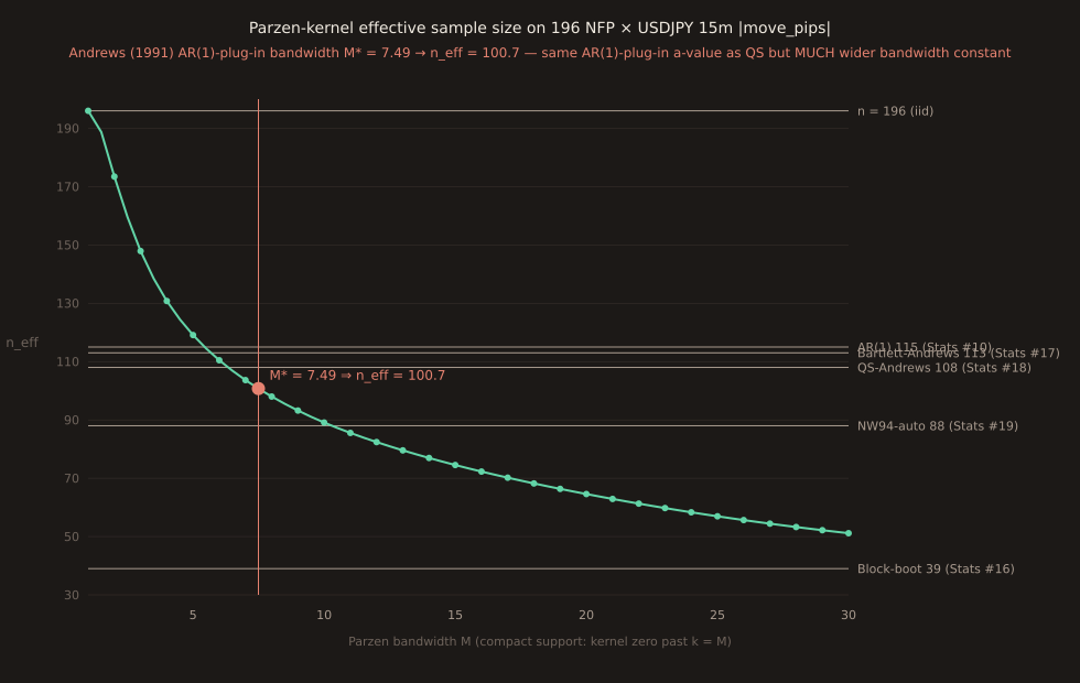
Fifth installment of the kernel-family arc on the same 196-release NFP × USDJPY 15m |move_pips| series (Stats #10 diagnosed the autocorrelation). Andrews (1991) Section 10 recommends Quadratic Spectral as the general-purpose HAC kernel and Parzen as the computational substitute (compact support means the sum truncates at k = M, O(M) work, whereas QS extends to all lags). Today: Parzen-kernel n_eff at Andrews-1991 optimum bandwidth M* = 7.49 is 100.75.
That’s 6.5% below QS (Stats #18’s 108), 11% below Bartlett (Stats #17’s 113), and 15% ABOVE the NW94-automatic Bartlett (Stats #19’s 88). Fifth leg of the kernel-family arc; ledger’s queued Parzen-Tukey-Hanning item is now marked PUBLISHED on the Parzen leg.
The Parzen kernel
Andrews (1991) equation 2.7 gives the Parzen kernel as a piecewise cubic:
K(u) = 2·(1 − |u|)³ for 1/2 < |u| ≤ 1
K(u) = 0 otherwise
Three key properties. Compact support: exactly zero at |u| ≥ 1, so the τ_int sum truncates at k = ceil(M) instead of extending to all lags like QS. That’s the “fast-QS” property Andrews notes as the reason to use Parzen when computational time matters. Continuous everywhere: both derivatives match at |u| = 1/2 (the piece-boundary) and the kernel is zero at |u| = 1 (the outer boundary), so no jump discontinuities. PSD-by-construction: guarantees a positive semi-definite HAC covariance matrix regardless of the sample autocorrelation profile (Andrews Section 2; a property shared with Bartlett and QS but NOT with Tukey-Hanning).
Andrews’ automatic bandwidth for Parzen
Same Andrews 1991 equations 5.3 and 5.9 as the QS post used — Parzen is a q=2 kernel too, so it shares the AR(1) plug-in formula with QS and Tukey-Hanning. Different bandwidth constant (2.6614 vs 1.3221), same functional form:
M* = 2.6614 · (a(2) · T)^(1/5)
On our sample (ρ(1) = 0.2601, T = 196):
M* = 2.6614 · (0.9029·196)^(1/5) = 2.6614·(176.97)^(1/5) = 2.6614·2.815 = 7.49
Parzen’s M* = 7.49 is roughly 2×QS’s S* = 3.72 on the same sample. The constant ratio 2.6614 / 1.3221 = 2.013 accounts for the fact that QS’s smoother spectral window puts nontrivial weight all the way out to k ≈ 3·S* while Parzen’s compact support cuts off hard at k = M — so Parzen needs a bigger nominal M to reach the same “effective bandwidth” QS achieves at smaller S.
The Parzen weight table at M* = 7.49
| k | k / M* | K_Parzen | ρ(k) empirical | contribution to τ_int |
|---|---|---|---|---|
| 1 | 0.1334 | 0.9074 | +0.2601 | +0.472 |
| 2 | 0.2669 | 0.6867 | +0.2441 | +0.335 |
| 3 | 0.4003 | 0.4233 | +0.0452 | +0.038 |
| 4 | 0.5338 | 0.2027 | +0.2120 | +0.086 |
| 5 | 0.6672 | 0.0737 | +0.0660 | +0.010 |
| 6 | 0.8007 | 0.0158 | +0.1333 | +0.0042 |
| 7 | 0.9341 | 0.0006 | +0.0584 | +0.00007 |
| ≥8 | ≥1.07 | 0 (cutoff) | — | 0 |
Sum of contributions = +0.9455. Doubled (for the ±k symmetry of the ACF) and added to the k = 0 term of 1: τ_int = 1 + 2·0.4726 = 1.9455. n_eff = 196 / 1.9455 = 100.75.
Two things worth noticing in the table. First, the k = 4 row: Parzen K(0.5338) = 0.2027 is now on the second piece of the piecewise definition (past |u| = 0.5), so it uses the2·(1−|u|)³shape. The transition from the first piece to the second is smooth (K = 0.75 at both u = 0.5− and u = 0.5+, as constructed). Second, the k ≥ 8 row: exactly zero contribution, unlike QS which keeps small positive/negative weights out at k = 10, 15 (Stats #18’s post walks through those). That’s the “compact support” property that makes Parzen’s O(M) computation faster than QS’s O(T).
The 5-method kernel-family arc, complete
| Method | n_eff | τ_int | Bandwidth | Nature |
|---|---|---|---|---|
| IID (ceiling) | 196 | 1.00 | — | Assumes zero autocorrelation |
| AR(1) formula (Stats #10) | 115 | 1.70 | — | Parametric; AR(1) shape assumption |
| Bartlett @ Andrews M* = 4.51 (Stats #17) | 113 | 1.74 | 4.51 | q=1, PSD, O(M) |
| QS @ Andrews S* = 3.72 (Stats #18) | 108 | 1.82 | 3.72 | q=2, PSD, O(T), Andrews-preferred |
| Parzen @ Andrews M* = 7.49 (today) | 101 | 1.95 | 7.49 | q=2, PSD, O(M), compact-support |
| NW94-automatic Bartlett (Stats #19) | 88 | 2.22 | 8.00 | Data-driven bandwidth, not AR(1)-plug-in |
| Block bootstrap @ b_opt = 4.98 (Stats #16) | 39 | 5.03 | 4.98 | Whole sampling distribution, not mean-variance |
The mean-variance HAC estimates monotonically decrease from AR(1) 115 down to NW94 88. Each new method catches slightly more autocorrelation than the previous — not by design but as an emergent property of the specific autocorrelation profile in this sample.
Parzen at 101 sits between QS (108) and NW94 (88). The QS gap is because Parzen’s bigger M* = 7.49 gives more weight to the empirical ρ(4) = 0.212 than QS at S* = 3.72 does. The NW94 gap is because NW94 uses the Bartlett kernel (linear taper, cuts to zero past k = m) at bandwidth m = 8 — Bartlett’s stricter taper at k = 4 (weight 0.556) beats Parzen’s (0.203) at that specific lag, but Bartlett misses ρ(6) = 0.133 entirely (weight 0) while Parzen catches a bit of it (weight 0.016 × 0.133 = +0.002 to τ_int).
Why Parzen instead of QS in practice
The Andrews (1991) Section 10 recommendation is: “use QS + automatic bandwidth as the default; fall back to Parzen if computational speed matters.” The reason Parzen is the sanctioned substitute is exactly its compact support: QS sums over all lags (O(T) work), Parzen truncates at k = M (O(M) work). On a T = 200 sample the difference is invisible — on a T = 100,000 tick-data series the difference matters.
Parzen also inherits QS’s PSD-by-construction property while Tukey-Hanning (also q=2, also compact-support) does not. So Parzen is the “safe fast-QS”: same efficiency rate, cheaper compute, guaranteed PSD covariance matrix. The cost is that it can be slightly more variable than QS in finite samples — the O(T^{-4/5}) rate is the same but the finite-sample MSE constant is marginally higher.
Practical CI-width implication
Using the same sample mean 38.19 pips and sd 37.66 pips from Stats #17, the 95% t-CI half-widths across our full kernel-family arc are:
AR(1) (n_eff = 115): ±6.93p width 13.85p
Bartlett-Andrews (113): ±7.00p width 14.00p
QS-Andrews (108): ±7.16p width 14.32p
Parzen-Andrews (101): ±7.40p width 14.81p (today)
NW94-automatic (88): ±7.94p width 15.88p
Block bootstrap (39): ±11.93p width 23.85p
The kernel-family spread is ±0.94p(13.85 to 15.88p) — a 15% widening from AR(1)’s asymptotic formula to NW94’s automatic Bartlett. Parzen at 14.81p sits almost exactly in the middle. The block bootstrap at 23.85p is 60-70% wider than any kernel HAC method — a reminder that the kernel-family question and the block-bootstrap question are targeting different quantities.
What this doesn’t say
The 5-method arc is not a hierarchy of correctness. AR(1) 115, Bartlett 113, QS 108, Parzen 101, NW94 88 are all defensible estimators of the same variance-of-the-mean quantity under different modeling assumptions and bandwidth-selection procedures. The monotone descent from 115 to 88 is a sample- specific feature of the NFP × USDJPY autocorrelation profile (moderate ρ(1), slow decay through ρ(2-6), a couple of small higher-lag echoes at ρ(11) and ρ(15)). On a different sample the ordering could easily be different.
Parzen is not always PSD-preferred over QS. Both are always PSD by construction. The reason to pick Parzen over QS is speed (O(M) vs O(T)) or storage. If neither constraint bites, QS is the theoretically-preferred kernel per Andrews Section 10. Parzen is a substitute, not an upgrade.
Higher-order kernel HAC has a Tukey-Hanning alternative(also q=2, also compact-support). It differs from Parzen in that it’s NOT guaranteed PSD. On today’s sample the PSD guarantee wouldn’t bite anyway (all four kernel estimates give positive n_eff) — but it can bite on samples with strongly-negative ρ(k) at intermediate lags. Ledger keeps Tukey-Hanning queued as a future installment for the “when the PSD guarantee actually matters in practice” angle.
The Andrews-Monahan 1992 pre-whitening extension— the natural closing installment of the HAC-history arc — takes a completely different approach: fit an AR(1) filter to the residuals BEFORE applying the HAC kernel, so the kernel has less autocorrelation to catch. Today’s Paper Trail #20 covers that paper as the complementary paper-side leg. The two go together: same sample, same authors’ theoretical arc, different points in the correction pipeline.
Not financial advice. Educational only.