Statistics for Traders #8: Sharpe ratio via the UK CPI × GBPJPY big-beat bucket — a +16-pip mean move looks great until you divide by 23 pips of noise
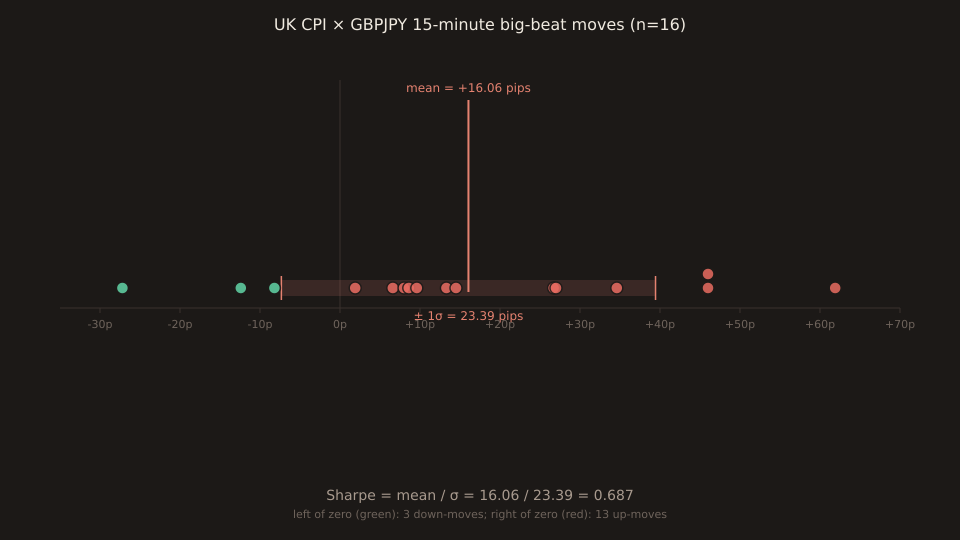
The 16 big-beat UK CPI prints on GBPJPY had a mean 15-minute move of +16.06 pips and a standard deviation of 23.39 pips. Divide the first by the second and you get the per-trade Sharpe ratio: 0.687. That’s the answer to “how much edge per unit of noise?” on this signal. Under the rule of thumb where annualized Sharpe below 1 is weak, 1-2 is decent, above 2 is exceptional: this signal, on this bucket, at this frequency, is weak.
Today’s slot-1 post found a clean 5-bucket walk for UK CPI on GBPJPY with 13 of 16 big-beat prints sending GBPJPY up (81% up-rate). Those are the same 16 prints this installment uses. The high up-rate LOOKS impressive, and the +11.45p median gets close to a real trading edge — but as we’ll see below, when you divide by the noise (23.39p standard deviation), the Sharpe ratio doesn’t survive the annualization multiplier for a signal that only fires twice a year.
The formula
Sharpe ratio = mean / standard deviation. Both are computed from your sample of trades. Both need to be in the same units. It’s dimensionally consistent — pips divided by pips leaves you with a pure number. That’s deliberate: Sharpe is designed so that a bond strategy’s Sharpe and an equity strategy’s Sharpe and an FX signal’s Sharpe are comparable on a single axis.
Some textbook treatments use (mean − risk_free_rate) / std— the numerator is “excess return”, the return above what you’d get by parking money in a Treasury. For a 15-minute FX event trade the risk-free rate over 15 minutes is effectively zero at any plausible short-rate level, so the two formulas agree here to the third decimal. For a multi-quarter buy-and-hold benchmark the distinction matters.
Worked example: UK CPI × GBPJPY big-beat, all 16 prints
The 16 individual 15-minute pips-moves, sorted:
-27.20 -12.40 -8.20 +1.90 +6.60 +8.00 +8.60 +9.60 +13.30 +14.50 +26.70 +27.00 +34.60 +46.00 +46.00 +61.90
Four-step calculation:
step 1 sum of moves = +256.90 pips step 2 mean = 256.90 / 16 = +16.06 pips step 3 Σ(move − mean)² / 15 = 547.06 sqrt(547.06) = 23.39 pips (standard deviation) step 4 Sharpe = 16.06 / 23.39 = 0.687 ← per-trade Sharpe
The per-trade Sharpe is 0.687. Under a normal-distribution interpretation, a mean 0.687 standard deviations above zero corresponds to about a 75% up-rate. The observed up-rate on this bucket is 81% — a touch higher than the Sharpe-implied normal rate, because the negative side of the distribution has a couple of large-magnitude outliers (the 2013-11-13, 2017-06-13, and 2023-03-22 prints) that pull the mean down disproportionately relative to how often the bucket goes down at all. This is the fat-tailed structure that Stats for Traders #6 (kurtosis) established generally.
Annualization: √n and why it matters
Per-trade Sharpe is a common intermediate output, but the finance-industry standard is annualized Sharpe — the per-trade number multiplied by √(trades per year). The √n scaling comes from the fact that variances of independent random variables add, so standard deviations add in quadrature. If you run n independent trades of the same edge, cumulative return scales linearly (n × mean) but cumulative std scales with √n (√n × std), so Sharpe scales with √n.
UK CPI publishes 12 times a year, but the bucket cutoff (surprise_z > +1.5) means only about 2 prints land in big_beat per year on average. A strategy that trades ONLY big-beat UK CPI prints on GBPJPY:
per-trade Sharpe = 0.687 trades per year = 2 (approx.) annualized Sharpe = 0.687 × sqrt(2) = 0.97
About 1 — the low end of “decent” and still well below the “exceptional” band. If instead you traded EVERY UK CPI print regardless of bucket (12/year), the per-trade edge collapses (miss and beat prints partly cancel in the pooled sample) and the annualized Sharpe drops further. The concrete lesson: which prints you trade matters more than how many. Two selective trades per year at a genuine edge is better than 12 arbitrary trades per year that dilute the signal.
Four assumptions Sharpe makes — all violated by FX data
1. IID: independent, identically-distributed returns. FX bucket returns are not IID. Volatility clusters (per Paper Trail #5 (Engle 1982 ARCH)) — periods of high variance produce sequential high-variance prints, and Sharpe treats them as though they came from a constant-variance distribution. And event returns aren’t independent across close dates: same-day contamination is filtered at the API level, but macro cycles within a month/quarter mean per-print returns aren’t genuinely independent.
2. Normality.Sharpe’s interpretation as a probability-of-winning metric assumes returns are normally distributed. FX bucket data is fat-tailed (see Stats #6). The “68% of trades within 1σ” rule of thumb doesn’t hold as advertised — you’ll see more outliers than a normal distribution predicts, in both directions.
3. Zero-cost execution.Sharpe doesn’t subtract commission, spread, or slippage. On a JPY cross the spread is typically 1.5-2 pips, so a 16-pip mean move nets to about 14 pips per round trip. Effective per-trade Sharpe drops from 0.69 to about 0.6. Any Sharpe you compute from raw pips-moves is an upper bound.
4. Constant risk-free rate. Proper Sharpe uses (return − risk_free_rate) / std. For 15-minute event trades this doesn’t matter (~0.0001% risk-free return over 15 minutes). For a buy-and-hold benchmark it does.
These four caveats don’t make Sharpe useless — they make it a comparative yardstick, not an absolute measure. Use it to rank signals against each other (JPY-cross big-beat vs USD-cross big-beat is a fair Sharpe comparison because both live in the same sample geometry). Don’t use it as a promise of realised P&L.
Cross-check: same event, same bucket, on GBPUSD
UK CPI × GBPUSD 15m big_beat (n=16): mean +14.24 p, std 26.56 p, per-trade Sharpe 0.536. The JPY cross has a slightly larger mean (16.06p vs 14.24p) and a smaller std (23.39p vs 26.56p), so its edge-per-unit-noise ratio comes out cleanly higher: 0.687 vs 0.536. That’s the amplification story from today’s slot-1 post made concrete: the JPY cross gives you a better ratio in both directions — bigger typical edge AND less variability around it — not just a bigger absolute pip move.
What’s next in the series
Sharpe fits alongside the earlier installments as follows: Stats #2 gave you std dev as a size-of-noise measure; Stats #3 (sample size, distribution-free CI for the median) and #7 (t-distribution CI for the mean) told you how confident to be in a point estimate; #4 (percentiles) and #5 (skew) and #6 (kurtosis) described the shape of the distribution beyond the mean and std; and Stats #1 (z-score) was the input-side equivalent (how big was the surprise on the release calendar). Sharpe is the FIRST installment that combines mean and std into a single unit-free tradability score. Upcoming: correlation vs causation (a worked FX example), autocorrelation (why 20 back-to-back candles don’t count as 20 observations), and bootstrap resampling for tail-bucket confidence intervals (flagged as the tool of choice back in Stats #7).
Open the tool → Free forever. No signup. No email required.